


Next: Phase-ray formulation
Up: Shragge and Biondi: Phase-rays
Previous: Shragge and Biondi: Phase-rays
The theory outlined in this section closely follows that of Foreman's
exact ray theory Foreman (1989), but is summarized here for completeness.
Ray theory may be used to compute the characteristics to the
time-independent, homogeneous Helmholtz equation,
| 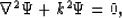 |
(1) |
where  is the desired wavefield solution, and k is the wavenumber.
In most ray theoretic developments, the wavefield is represented by an
ansatz solution,
is the desired wavefield solution, and k is the wavenumber.
In most ray theoretic developments, the wavefield is represented by an
ansatz solution,  , where
  and
and  are the
amplitude and phase functions, respectively.
Substituting this representation into the Helmholtz equation yields
the usual eikonal and transport equations,
are the
amplitude and phase functions, respectively.
Substituting this representation into the Helmholtz equation yields
the usual eikonal and transport equations,
| 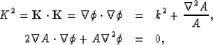 |
(2) |
| |
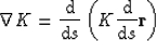
where  is the phase gradient vector (see figure
 ![[*]](http://sepwww.stanford.edu/latex2html/cross_ref_motif.gif) ).
).
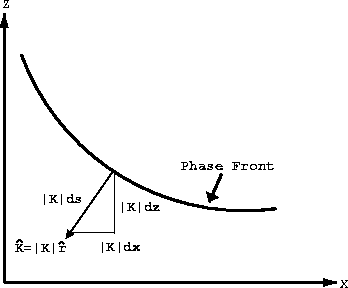
Rays
Figure 1 Schematic of phase-front gradient
quantities. is the phase gradient vector,
 is the gradient magnitude along step is the gradient magnitude along step  , and , and  and and  are the projections of along the x and z
coordinates, respectively. are the projections of along the x and z
coordinates, respectively.
|
|  |

Solutions to equations (2) are the ray paths and
the amplitudes along these ray paths, respectively.
In isotropic media the gradient of the phase function,
 , is orthogonal to surfaces of constant phase and
represents the instantaneous direction of propagation.
Explicitly, this may be written,
, is orthogonal to surfaces of constant phase and
represents the instantaneous direction of propagation.
Explicitly, this may be written,
| 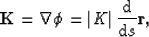 |
(3) |
where is an element of length, and  is a vector element
of the ray-path.
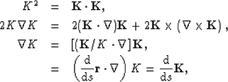
A ray-path equation is developed by taking the gradient of the
phase gradient magnitude (i.e.
is a vector element
of the ray-path.
A ray-path equation is developed by taking the gradient of the
phase gradient magnitude (i.e.  ),
),
|  |
|
| |
| (4) |
| |
where  has been
employed.
Using equation (3) this may be written explicitly,
has been
employed.
Using equation (3) this may be written explicitly,
|  |
(5) |
Coupling between the eikonal and transport equations is evident
through the dependence of the eikonal equation on amplitude function, A.
In many cases a high-frequency approximation (i.e.  ) is used to decouple these equations.
Use of this approximation yields the usual form of the ray path equation,
) is used to decouple these equations.
Use of this approximation yields the usual form of the ray path equation,
|  |
(6) |
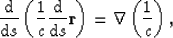
where c is the velocity.
Use of this approximation also eliminates the frequency dependence of
ray trajectories (see Appendix A).
One manner of reintroducing frequency-dependent ray trajectories is
discussed in a latter section.