Simulated Annealing

Simulated Annealing is a non-linear optimization method. The idea is to find the global minimum in a way similar to cooling magma forming crystals. If the magma cools too quickly, glass forms. Glass represents local minima. When the magma is cooled slowly enough, then crystal forms. Crystal represents global minima. Rothman used this approach for statics estimation Rothman (1985).

We can define our optimization goal as:

 

$${\bold E}\bold{_1}= \sum_{i}{\bold C}(m_i)$$ (1)

For this problem, we needed to apply some sort of regularization to ensure that the solution is smooth.  

$${\bold E}\bold{_2}= \sum_i \rm abs( \frac{\rm d}{\rm dt}\rm{\bold m}\rm)$$ (2)

These two equations can be combined and balanced with $\epsilon$ as  

$${\bold E}= {\bold E}\bold{_1}+\epsilon {\bold E}\bold{_2}$$ (3)

A computation template for the method of simulated annealing is

 

		 $\bold{rate= f\ (iteration) \quad\longleftarrow\quad} \rm{define \ cooling \ schedule}$		 $\bold m \quad\longleftarrow\quad\bold {0.}$		 iterate { 
		 		  $\bold {n} \quad\longleftarrow\quad{\rm random\ numbers}$ 
		 		  if  $\bold {E_{n}} < \bold {E_m}\ \{$		 		 		$\bold m \quad\longleftarrow\quad\bold {n}$		 		  $\}\rm \ else\ \{$		 		 		 $\bold P =e^{-\Delta \bold E \cdot \bold{rate}}$		 		 		$\}$ 
		 		  if  $\bold {P} \gt \rm random\ number \ \{$		 		 		$\bold m \quad\longleftarrow\quad\bold {n}$ 
		 		 		$\}$ 
 
		 		 } 

The model ($\bold m$) is a vector which defines the extracted lags from the cross-correlagram ($\bold C$). Energy ($\bold E$) is what we are trying to minimize by finding the smoothest path with the lowest energy across the cross-correlagram. The trial model ($\bold {n}$) is a vector the same size as $\bold m$.We define a $\bold {rate}$ parameter to follow a cooling schedule as a function of iterations. A computation template for the method of simulated annealing is $\bold P$,a probability value assigned to a trial vector ($\bold {n}$). If a random value is less than this probability value, the trial vector will be accepted even if it has a larger energy. This will allow the solution to escape local minima. This is analogous to cooling magma; when the temperature is high, it is less likely to get locked into position. As the number of iterations increases, $\bold P$ becomes smaller, making it less likely to accept a solution with greater energy. If the rate is sufficiently small, this method should converge to the global minimum.

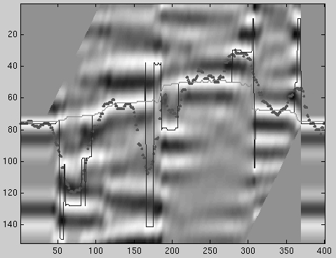
I applied this method to estimate fault slip. The result is in Figure 9. The dots represent the annealing solution. The initial guess for $\bold m$ was the maximum, the solid line. This required numerous iterations and, although it appears that it may be heading toward convergence (the light solid line), it may not be. In fact, the added complication of the $\epsilon$ parameter makes it quite likely to converge to a flat model. The regularization is causing the slow convergence because randomly changing model points tend to cause an extremely unsmooth solution. Therefore, the regularization part is throwing out most of the possible solutions because they are too rough.

 

Anneal1bw
Figure 9 Simulated Annealing result after many iterations, dots. Heavy solid line, picked maximum initial solution. Light solid line, desired result.