Selecting reference velocities

Lloyd's methods translate fairly easily for a reference velocity selection problem. The values become velocities, the centroids become the reference velocities, and the cells are regions with the same reference velocity. For selecting the initial reference velocities, I used evenly spaced quantiles of the velocity. At early iterations I replace step 3 of Lloyd's method by something a bit more complex.

3a

Remove cells whose centroids are closer than a certain percentage from its neighbors (typically 3-8%).

3b

Remove cells with fewer than a given number of points (typically 1-3%).

3c

Given the removed points in steps 3a and 3b, find the regions with the highest variance that are a given distance away from its neighbors. If no regions meeting these criteria are found, remove them.

The purpose of modifying Lloyd's method is to attempt to avoid local minima. Regions whose centroid are close to its neighbor, or are sparsely populated, are replaced by splitting up regions that seem to be least accurately described by their current centroid.

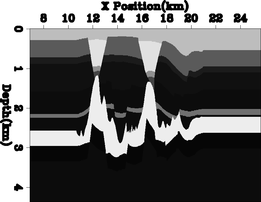VELOCITY SELECTION TESTS To test the methodology I applied it to several different velocity models. The first model is a 2-D synthetic, provided by BP, attempting to emulate North Sea geology (Figure 2). The model is composed of several constant velocity layers. For this test I used the entire velocity model as an input, even though when doing migration each depth step will by analyzed independently. Figure 3 shows a histogram of the velocity function overlayed by the initial reference velocities (0) and those after five (5) and twenty iterations (*). Note how all of the major velocities are identified by the method.

 

amoco-vel Figure 2 A 2-D synthetic velocity model made up of constant velocity layers.

 

amoco-hist-overlay Figure 3 A histogram of the velocity function overlayed by the initial reference velocities (0) and those after five (5) and twenty iterations (*).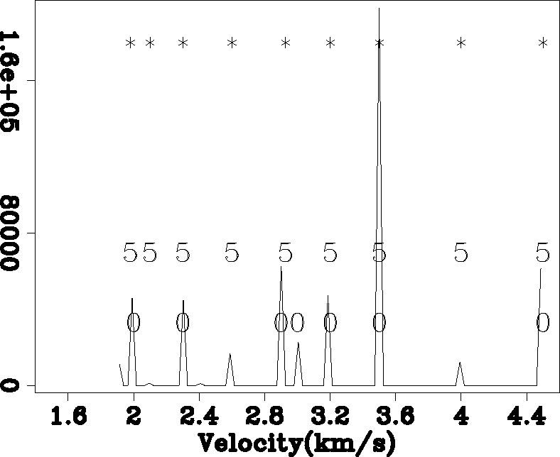

For the second example I smooth the velocity in Figure 2 to obtain the velocity in Figure 4. Figure 5 shows the selected velocities. Note how the initial velocities were clustered around 3.6 km/s. The final velocities are generally more spread out, closer in velocity ranges with high count. Also note that in each region the velocity that is most common is chosen as a reference.

 

amsm-vel Figure 4 A smoothed version of the model in Figure 2.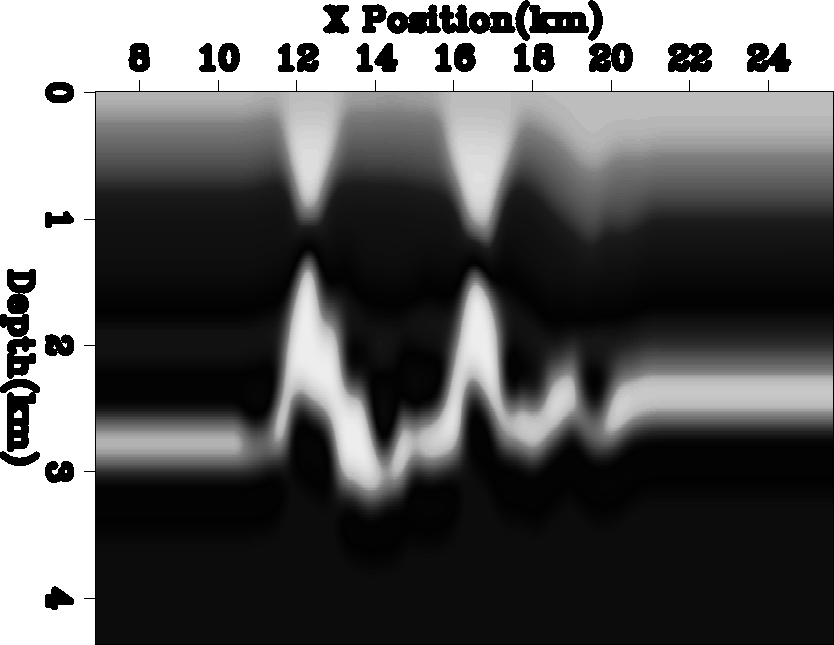

 

amsm-hist-overlay Figure 5 A histogram of the velocity function in Figure 4 overlayed by the initial reference velocities (0) and those after five (5) and twenty iterations (*).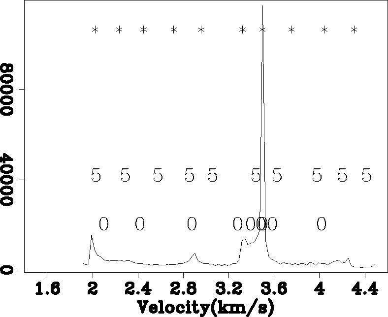

To test the method's ability on functions with bimodal distributions (such as regions with salt), I used the upper (Figure 6) and lower (Figure 8) portion of the SMAART JV Sigsbee synthetic. Figures 7 and 9 show the selected velocities. Note how in each example the method determined that fewer reference velocities were needed. In each case a single reference velocity between the two modes of the distribution (this reference velocity was kept because some velocities still fall in this region).

 

zig1-vel Figure 6 The top portion of the Sigsbee synthetic.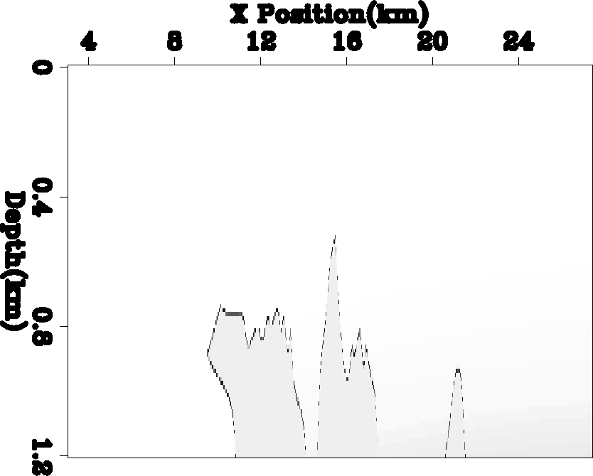

 

zig1-hist-overlay Figure 7 A histogram of the velocity function in Figure 6 overlayed by the initial reference velocities (0) and those after five (5) and twenty iterations (*).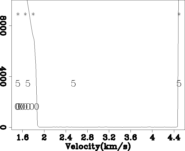

 

zig2-vel Figure 8 The bottom portion of the Sigsbee synthetic.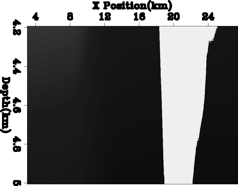

 

zig2-hist-overlay Figure 9 A histogram of the velocity function shown in Figure 8 overlayed by the initial reference velocities (0) and those after five (5) and twenty iterations (*).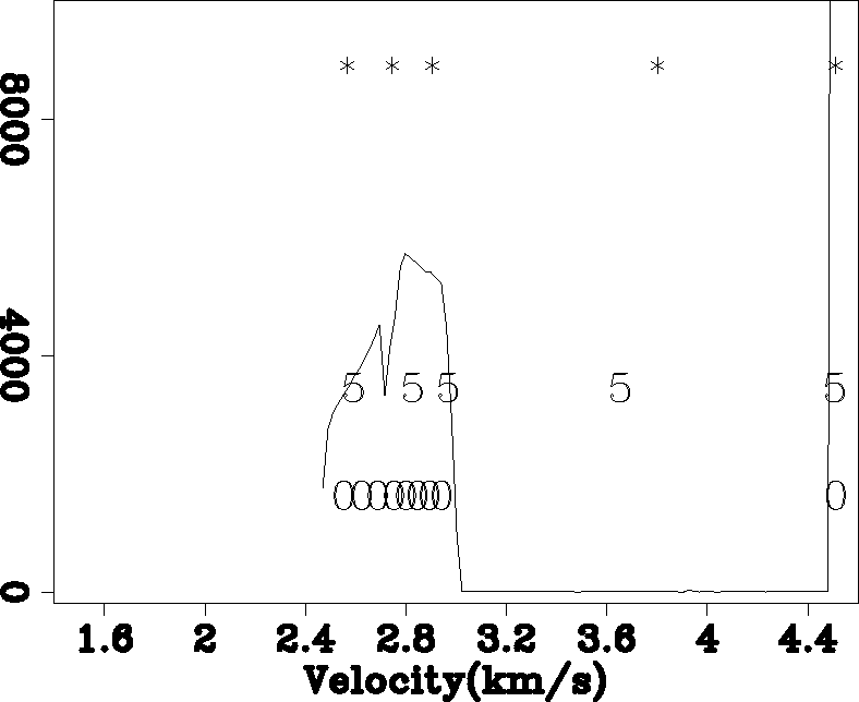