


Next: Stronger lateral velocity variations?
Up: Biondi: Midpoint-offset reverse-time migration
Previous: Introduction
We would like to propagate
the recorded wavefield
backward in time instead of downward into the Earth,
but we also would like to preserve the computational advantages of
propagating the recorded wavefield in
midpoint-offset coordinates.
The advantage of the midpoint-offset coordinates
derives from the focusing of the reflected wavefield towards zero offset
as it approaches the reflector.
The wavefield focuses towards zero-offset during downward continuation
because we are essentially datuming the whole data set to
an increasingly deeper level in the Earth.
It is thus reasonable to start our derivation
from the double square root (DSR) equation,
that is the main tool for datuming prestack data.
As we will see later, this choice of a starting point
limits the usefulness of the final result.
The DSR equation in the frequency-wavenumber
domain is
|  |
(1) |
where  is the temporal frequency, kxs and kxg
are respectively the wavenumber associated to the
source and receiver locations, and
is the temporal frequency, kxs and kxg
are respectively the wavenumber associated to the
source and receiver locations, and  and
and  are the slowness at the source and receiver locations.
We first start by rewriting the DSR in terms of midpoint xm
and half offset xh as
are the slowness at the source and receiver locations.
We first start by rewriting the DSR in terms of midpoint xm
and half offset xh as
|  |
(2) |
where kxm and kxh
are respectively the wavenumber associated to the
midpoint xm and the half-offset xh.
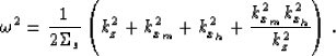
Then,
to obtain a time marching equation,
we first square
equation (2) twice and rearrange the terms
into:
|  |
(3) |
where
| 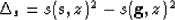 |
(4) |
| 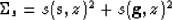 |
(5) |
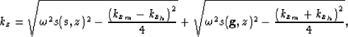
Equation (3)
is a second order equation in  .It has another solution
in addition to the desired one.
It can be greatly simplified by assuming
.It has another solution
in addition to the desired one.
It can be greatly simplified by assuming
 .Then
equation (3) can be rewritten as
.Then
equation (3) can be rewritten as
|  |
(6) |
This is the basic equation solved for the numerical examples
shown in this paper.
Notice that when kxh is equal to zero,
equation (6) degenerates
to the well-known equation used
for reverse-time migration of zero-offset data
Baysal et al. (1984).
There are few alternatives on how to solve
equation (6) numerically.
The simplest one is to use finite-differences for approximating
the time derivative,
and Fourier transforms for evaluating the spatial-derivative operators.
Because the slowness term  is outside the parentheses
in equation (6),
using Fourier transforms does not preclude the use
of a spatially variable slowness field.
Strong lateral velocity variations would cause
problems because of the approximations needed to go
from equation (3) to
equation (6),
not because of the numerical scheme used
to solve equation (6).
is outside the parentheses
in equation (6),
using Fourier transforms does not preclude the use
of a spatially variable slowness field.
Strong lateral velocity variations would cause
problems because of the approximations needed to go
from equation (3) to
equation (6),
not because of the numerical scheme used
to solve equation (6).
The time marching scheme that I used can be summarized
as;
|  |
(7) |
Using a Fourier method
to evaluate the spatial-derivative operators,
makes it easy to handle the real limitation
of equation (6);
that is,
the presence of the vertical wavenumber kz
at the denominator.
Waves propagating horizontally have an effective infinite velocity,
making a finite-difference solution unstable,
no matter how small the extrapolation time step.
Unfortunately,
this is a major obstacle
for migrating overturned events,
which is one of the main goals for developing
a reverse time migration in midpoint-offset coordinates.
The problem exists only for finite offset data ( ).
In retrospective, the occurrence of problems
for waves that overturn at finite offset should not be surprising.
Equation (6)
was derived from the DSR
that cannot model data for which the source leg
overturns at different depth than the receiver leg.
).
In retrospective, the occurrence of problems
for waves that overturn at finite offset should not be surprising.
Equation (6)
was derived from the DSR
that cannot model data for which the source leg
overturns at different depth than the receiver leg.
For non-overturning events the problem can be sidestepped.
The spatial wavenumbers are related to
the reflector geological dip angle  and the aperture angle
  by the relationship
| 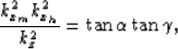 |
(8) |
By simple trigonometry is also possible to show
that for non-overturned events
| 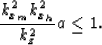 |
(9) |
In the Fourier domain
it is straightforward to include condition (9)
in the time-marching algorithm
and thus to avoid instability without suppressing
reflected energy.
Next: Stronger lateral velocity variations?
Up: Biondi: Midpoint-offset reverse-time migration
Previous: Introduction
Stanford Exploration Project
6/7/2002