Initial errors

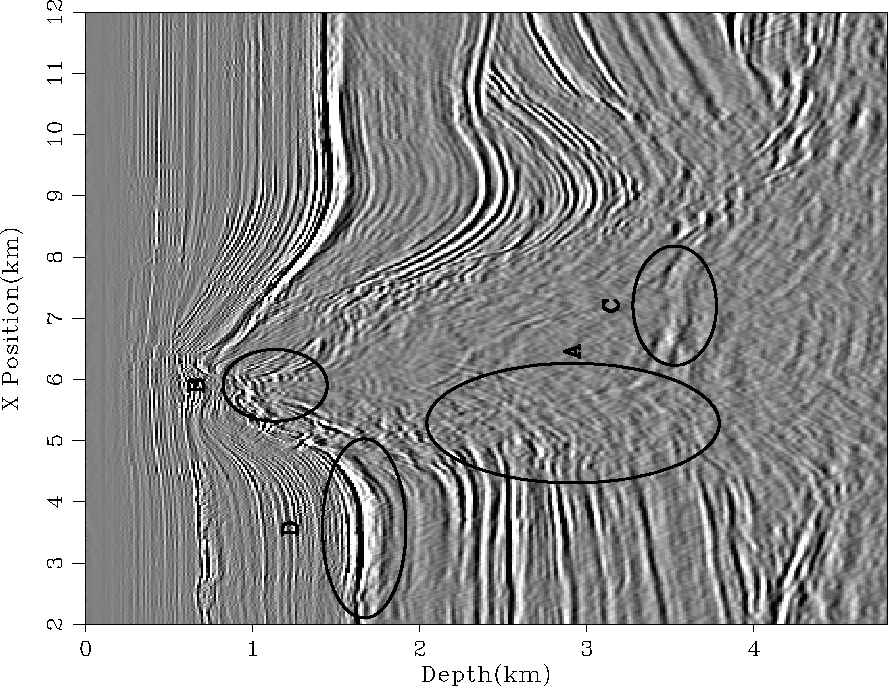
Figure 3 is result of migrating the data with the velocity of Figure 2. The strong chalk reflection ('D') is low frequency and focusing problems make its amplitude suspiciously space-variant. The salt is generally poorly defined. The salt top reflection (`B') is discontinuous. The bottom of the salt (`C') is poorly imaged. 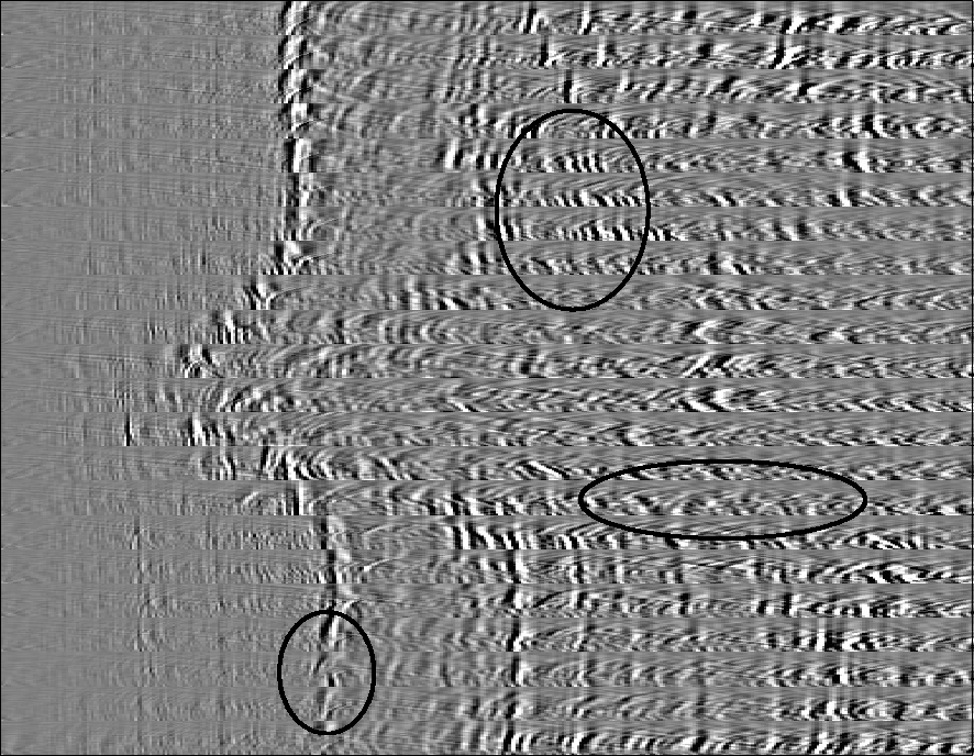The most interesting problem is along the salt edge (`A') where we see little reflector continuity below 2.8 km. If we look at the CRP gathers (Figure 4) we see significant moveout and focusing problems.

 

elf-mig0
Figure 3 Migration result using the velocity from Figure 2. Migrations problems can be seen at locations A-D.

 

moveout-vel0
Figure 4 Every 20th CRP gather from the initial migration. The circled areas show either focusing or or moveout problems.

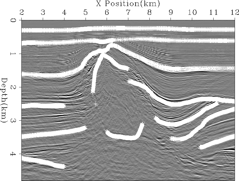
Using the initial migrated image I chose 11 reflectors to perform tomography with (Figure 5). To constrain the upper portion of the model I chose the water bottom reflection and two reflectors above the salt. I picked the salt top and salt bottom and three reflectors on both sides of the salt body.

 

overlays
Figure 5 Initial migration with picked reflectors overlaid.

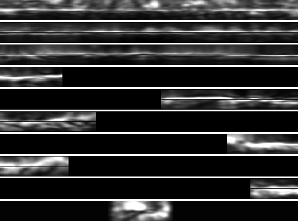
I performed moveout analysis using equation (). I selected the semblance at each reflector, Figure 6, and found a smooth curve using fitting goals (). The top two reflectors have have almost no moveout errors and the third reflector very little. The remaining reflectors all have some residual moveout errors that tomography can attempt to resolve.

 

elf-sem-ref.vel0
Figure 6 Semblance panels from ten of the reflectors used in the tomography. Note that that the top two reflectors are generally flat. The third reflector shows minimal moveout and the remaining reflectors still have significant residual moveout.