|
|
|
|
Modeling data error during deconvolution |
 (so the minus sign is missing
from all the analysis and code).
(so the minus sign is missing
from all the analysis and code).
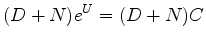
The decon filter  , parameterized by
  , we take as noncausal.
The constraint is no longer a spike at zero lag,
but a filter whose log spectrum vanishes at zero lag,
, we take as noncausal.
The constraint is no longer a spike at zero lag,
but a filter whose log spectrum vanishes at zero lag,
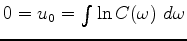 ,
so we are now constraining the mean of the log spectrum.
This is a fundamental change which we confess to being somewhat mysterious.
,
so we are now constraining the mean of the log spectrum.
This is a fundamental change which we confess to being somewhat mysterious.
The single regression for
including noise  now becomes two.
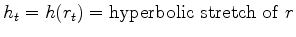
The notation  means the data fitting is done under a hyperbolic penalty function.
The regularization need not be
means the data fitting is done under a hyperbolic penalty function.
The regularization need not be  .
To save clutter I leave it as
until the last step
when I remind how it can easily be made hyperbolic.
.
To save clutter I leave it as
until the last step
when I remind how it can easily be made hyperbolic.
Under the constraint of a causal filter with  ,
traditional auto regression for
,
traditional auto regression for
 with its regularization looks more like
solved our non-minimum phase problem,
and seeing sea swell in our estimated shot wavelets
told us we need to replace  by
by  .
.
Antoine noticed the quasi-Newton method of data fitting requires gradients
but not knowledge of how to update residuals
 so the only thing we really need to think about is getting the gradient.
The gradient wrt
is the same as before (Claerbout et al. (2011))
except that
replaces
.
The gradient wrt
is the new element here.
so the only thing we really need to think about is getting the gradient.
The gradient wrt
is the same as before (Claerbout et al. (2011))
except that
replaces
.
The gradient wrt
is the new element here.
Let  ,
,  , and
, and  be time functions (data, noise, and filter).
Let
be time functions (data, noise, and filter).
Let
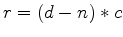 be the residual.
Let
be the residual.
Let
 .
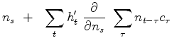
Expressing our two regressions in the time domain we minimize
.
Expressing our two regressions in the time domain we minimize
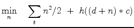 |
(5) |
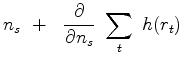
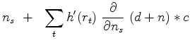
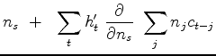
Now we go after the gradient, the derivative of the penalty function wrt each component of noise  .
Let the derivative of the penalty function
.
Let the derivative of the penalty function  wrt its argument
  be
called the softclip and be denoted
be
called the softclip and be denoted
 .
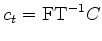
Let
.
Let  denote the FT of
  .
Let
.
Let  be the time reverse of
  while in Fourier space
 is the conjugate of
  .
.
 |
 |
 |
(6) |
|
 |
(7) | |
|
 |
(8) | |
|
 |
(9) | |
|
 |
(10) | |
|
 |
(11) | |
 |
|
 |
(12) |
.
Change
 to
to
 .
.
Now having the gradient we should be ready to code.
|
|
|
|
Modeling data error during deconvolution |