Computational analysis of extended full waveform inversion

Conventional FWI

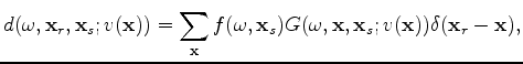
For conventional full waveform inversion, the modeled data is computed using the nonlinear forward operator as:

$$d(\omega, \mathbf x_r, \mathbf x_s; v(\mathbf x)) = \sum_{\mathbf... ...(\omega, \mathbf x, \mathbf x_s; v(\mathbf x)) \delta(\mathbf x_r - \mathbf x),$$ (1)

where $d(\omega, \mathbf x_r, \mathbf x_s; v(\mathbf x))$ is the modeled data, $v(\mathbf x)$ is the velocity model, $f(\omega, \mathbf x_s)$ is the source function, $\omega$ is frequency, $\mathbf x_s$ and $\mathbf x_r$ are the source and receiver coordinates, and $\mathbf x$ is the model coordinate. 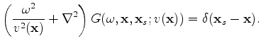In the acoustic, constant-density case, the Green's function $G(\omega, \mathbf x, \mathbf x_s; v(\mathbf x))$ satisfies:

$$\left( \frac{\omega^2}{v^2(\mathbf x)} + \nabla^2 \right) G(\omega, \mathbf x, \mathbf x_s; v(\mathbf x)) = \delta(\mathbf x_s - \mathbf x).$$ (2)

The propagation can be done in the time domain by convolving each model point with a finite-difference stencil. However, the time marching requires the time axis sampling to satisfy dispersion and stability conditions (Marfurt, 1984), generally much finer than the data sampling. Moreover, each time step requires multiplying the time slice by the velocity squared. Therefore, the cost of forward modeling can be written as:

$$C_{\rm FWI-F} = N_x N_y N_z N_{\rm source} (N_{tp} C_{\rm FDTD} + N_{tp}),$$ (3)

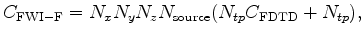
where $N_x$ , $N_y$ and $N_z$ , are the number of points along the three spatial axes, $N_{\rm source}$ is the number of sources, $C_{\rm FDTD}$ is the cost of convolving one model location by the time-domain finite-difference stencil and $N_{tp}$ is the number of time samples for propagation. By linearizing equation 1 over the squared slowness, we can compute the adjoint as:

$$\Delta s^2(\mathbf x) = \sum_{\omega, \mathbf x_r, \mathbf x_s} \... ... x_r; v(\mathbf x)) \Delta d^*(\omega, \mathbf x_r, \mathbf x_s; v(\mathbf x)),$$ (4)

where $\Delta s^2(\mathbf x)$ is the perturbation in squared slowness and $^*$ denotes the complex conjugate. For the adjoint, the imaging time sampling can be much larger than that of propagation since it does not need to satisfy the dispersion and stability conditions. Hence, the cost of computing the adjoint of FWI can be written as:

$$C_{\rm FWI-A} = N_x N_y N_z N_{\rm source} (2 \times N_{tp} C_{\rm FDTD} + 2 \times N_{tp} + N_{ti}),$$ (5)

where $N_{ti}$ is the number of time samples for imaging. The total cost of one iteration of FWI becomes

$$C_{\rm FWI} = N_x N_y N_z N_{\rm source} (6 \times N_{tp} C_{\rm FDTD} + 6 \times N_{tp} + N_{ti}).$$ (6)

Computational analysis of extended full waveform inversion