Integral operator quality from low order interpolation or Sometimes nearest neighbor beats linear interpolation

Examples

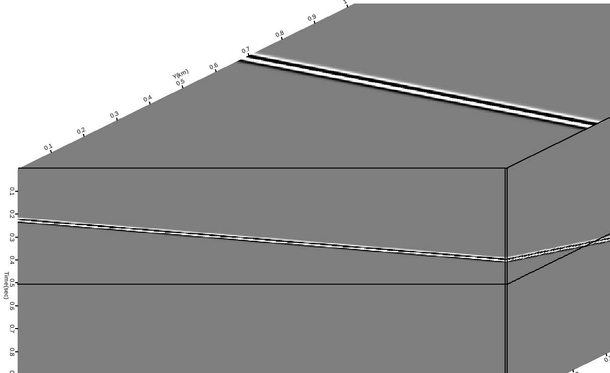
For my first example I created a dipping planar synthetic with a Ricker wavelet on it. (Figure 4) This $26.556^\circ$ dip is at an azimuth of $67.44^\circ$ and the central frequency of the Ricker wavelet is 64.22 Hz, slightly more than half the Nyquist frequency. The wavelet was imposed by calculating the analytic Ricker formula directly onto the trace samples and not by post-convolving a spike trace synthetic.

dipsynth Figure 4. Dipping 3D synthetic used for slant stack test.

I then did an areal slant stack along the same dip and azimuth as the plane with the output at the location of the first inline and crossline trace. I used nearest neighbor interpolation for this slant stack. Figure 5 shows the result overlain with what a perfect slant stack would have produced. Quite a respectable result even without spectral reshaping. (When spectral compensation is included, the result of nearest neighbor interpolation is nearly perfect as shown in Fig. 7.) Figure 6 shows the corresponding output for linear interpolation which, indeed, is not as accurate, agreeing with the analysis above.

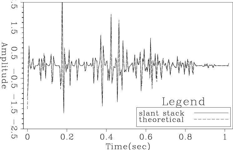
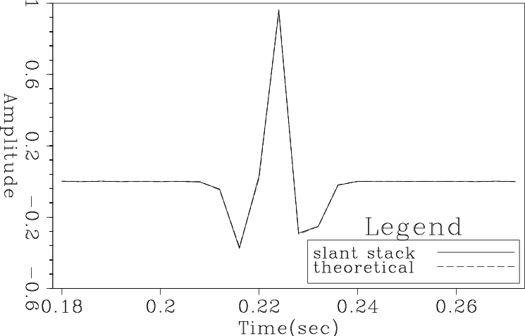
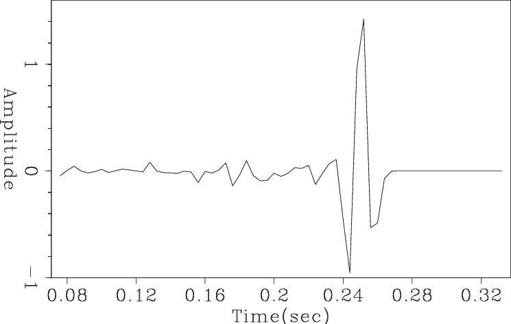
sstacknn Figure 5. Comparision of the perfect theoretical result with the output of slant stacking the data in Fig. 4 parallel to the planar event using nearest-neighbor interpolation.

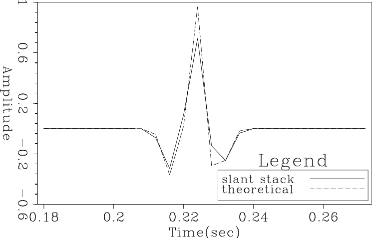
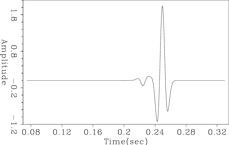
sstacklin Figure 6. Comparision of the perfect theoretical result with the output of slant stacking the data in Fig. 4 parallel to the planar event using linear interpolation.

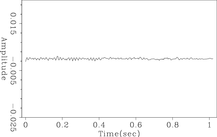
sstackspectnn Figure 7. Comparision of the perfect theoretical result with the output of slant stacking the data in Fig. 4 parallel to the planar event using nearest-neighbor interpolation followed by spectral compensation with the reciprocal of formula 1.

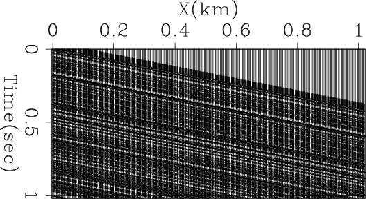
Of course, field data have many events, not just one, and summation operations will generally involve both constructive and destructive summation. Taking a first look at this topic, I modified the planar synthetic to have about 75 uniformly distributed individual parallel plane arrivals with amplitudes constructed according to a Gaussian distribution. (Figure 8.) Using this synthetic, I deliberately slant stacked horizontally (Fig. 10 which requires no interpolation) and again at a dip that was not parallel to the plane of the synthetic. (For Fig. 11 I opted to interchange the X and Y axis dips.) It is clear that nearest-neighbor interpolation created just about as much destructive cancellation as one would expect from a high order interpolation.

simpleranddip Figure 8. First slice of dipping 3D synthetic with sparse reflectors and Gaussian amplitude distribution used for slant stack test.

Nearest neighbor slant stack parallel to that dip yielded the expected high quality result show in Figure 9. Stacking horizontally, which requires no interpolation, or (destructive) slant stacking along a plane oriented with the X and Y axis interchanged resulted in equally small output amplitudes (a fraction of a percent) as expected.

sstackrandnn16 Figure 9. Comparision of nearest neighbor and high order interpolation slant stacking the data in Fig. 8 parallel to the planar event using nearest-neighbor interpolation followed by spectral compensation with the reciprocal of 1.

hstackrandnn Figure 10. Horizontal stack of the data in Fig. 8 gained by a factor of 100 over that in Fig. 9.

dstackrandnn Figure 11. Slant stack over a non-parallel direction of the data in Fig. 8 gained by a factor of 100 over that in Fig. 9.

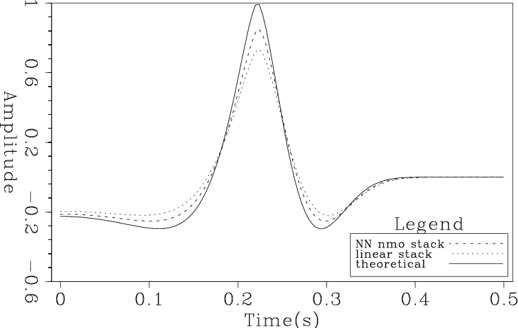
My second example is another situation where summation is expected to be almost exclusively constructive: 3D normal moveout. Figure 12 shows the result of applying NMO stack to a synthetic (flat dip) 3D CDP with maximum offsets of 12.8 and 25.6 km in the X and Y directions respectively. No spectral reshaping is shown because those results almost perfectly overlay their inputs. This anomaly arises because of NMO stretch which changes the shapes of the waveforms being stacked. In field data statics, deconvolution, and AVO effects will further modify the input waveforms, making spectral compensation analysis complicated and data dependent.

NMO3dcombo Figure 12. NMO stack comparison of nearest-neighbor, linear and high order interpolaton. Here no spectral compensation has been applied.

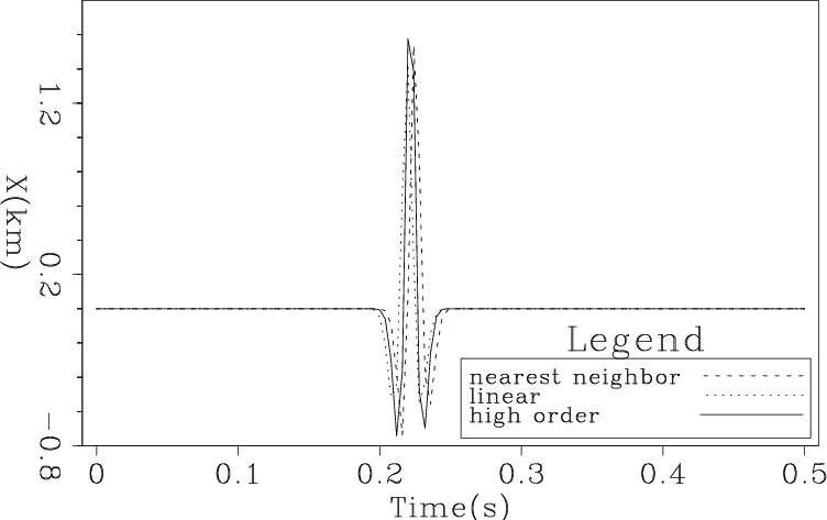
Closely related to NMO stack is common reflection surface (CRS) imaging which estimates and sums over prestack specular reflection surfaces (Jäger et al., 2001; Hertweck et al., 2004). I generated and CRS processed a prestack synthetic for a dipping plane and got the result in Figure 13. With the exception of an apparent one sample shift, probably a small coding bug, again nearest-neighbor did a fine job and outperformed linear linear interpolation.

Prestack3Dcombo Figure 13. CRS zero-offset trace for a dipping planar synthetic using nearest neighbor, linear and high-order interpolation.

Transitioning further into the balance between constructive and destructive interference, for a fourth example, I poststack migrated the synthetic of Fig. 4 with the same constant velocity used to create it. Using nearest-neighbor interpolation, the output at the first inline and crossline trace location is shown in Figure 14. Linear interpolation produces Figure 15 and highly accurate interpolation produces 16. In this case, increasing the order of the interpolant does increase accuracy, however the level of residual artifact is disconcerting.

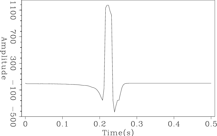
mig3Dnn Figure 14. Poststack 3D Kirchhoff time migration of the dipping planar synthetic using just nearest-neighbor interpolation.

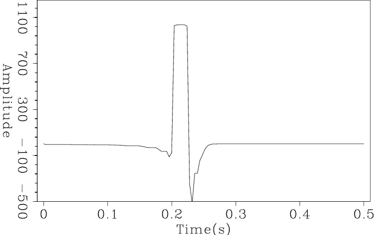
mig3Dlin Figure 15. Poststack 3D Kirchhoff time migration of the dipping planar synthetic using linear interpolation.

mig3Dnn16 Figure 16. Poststack 3D Kirchhoff time migration of the dipping planar synthetic using high-order interpolation.

The fundamental difference between the last example and the previous ones is that poststack Kirchhoff migration sums only a few samples coherently to form an image point sample. With prestack Kirchhoff, however, the number of coherent samples forming an image point sample is much larger. Figures 17 and 18 show 3D prestack Kirchhoff migration of a horizontal planar event. (Couldn't get the dipping plane version working in time.) There is no longer annoying precursor noise in these results.

Kirchnn Figure 17. Prestack 3D Kirchhoff time migration of a horizontal planar synthetic using just nearest-neighbor interpolation. No attempt was made to taper aperture or apply phase corrections.

Kirchlin Figure 18. Poststack 3D Kirchhoff time migration of a horizontal planar synthetic using linear interpolation. No attempt was made to taper aperture or apply phase corrections.

Integral operator quality from low order interpolation or Sometimes nearest neighbor beats linear interpolation