PIXEL-PRECISE VELOCITY SCANNING

Traditionally, velocity scanning is done by the loop structure given in chapter , in which the concept of a velocity transform was introduced.

This structure is

   do v
       do tau
           do x
               t = sqrt( tau**2 + (x/v)**2 )
               velo( tau, v) = velo( tau, v)  +  data( t, x)

These loops transform source-receiver offset x to velocity v in much the same way as Fourier analysis transforms time to frequency. Here we will investigate a new alternative that gives conceptually the same result but differs in practical ways. It is to transform with the following  loop structure:

do tau
    do t = tau, tmax
        do x
            v = sqrt( x**2  / ( t**2 - tau**2 ))
            velo( tau, v) = velo( tau, v)  +  data( t, x)

Notice that $t = \sqrt{\tau^2+(x/v)^2}$ in the conventional code is algebraically equivalent to $v=x/\sqrt{t^2-\tau^2}$ in the new code. The traditional method finds one value for each point in output space, whereas the new method uses each point of the input space exactly once.

The new method, which I have chosen to call the ``pixel-precise method,''

differs from the traditional one in cost, smoothing, accuracy, and truncation. The cost of traditional velocity scanning is proportional to the product N_t N_x N_v of the lengths of the axes of time, offset, and velocity. The cost of the new method is proportional to the product N_t² N_x/2. Normally N_t/2 > N_v, so the new method is somewhat more costly than the traditional one, but not immensely so, and in return we can have all the (numerical) resolution we wish in velocity space at no extra cost. The verdict is not in yet on whether the new method is better than the old one in routine practice, but the reasoning behind the new method teaches many lessons. Not examined here is the smooth envelope (page ) that is a postprocess to conventional velocity scanning.

 

lineint Figure 1 A typical hyperbola crossing a typical mesh. Notice that the curve is represented by multiple time points for each x.

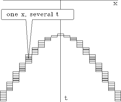
Certain facts about aliasing must be borne in mind as one defines any velocity scan. A first concern arises because typical hyperbolas crossing a typical mesh encounter multiple points on the time axis for each point on the space axis. This is shown in Figure 1. An aliasing problem will be experienced by any program that selects only one signal value for each x instead of the multiple points that are shown. The extra boxes complicate traditional velocity scanning. Many programs ignore it without embarrassment only because low-velocity events contain only shallow information about the earth. (A cynical view is that field operations tend to oversample in offset space because of this limitation in some velocity programs.) A significant improvement is made by summing all the points in boxes. A still more elaborate analysis (which we will not pursue here) is to lay down a hyperbola on a mesh and interpolate a line integral from the traces on either side of the line.

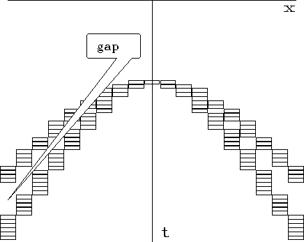
A second concern arises from the sampling in velocity space. Traditionally people question whether to sample velocity uniformly in velocity, slowness, or slowness squared. Difficulty arises first on the widest-offset trace. When jumping from one velocity to the next, the time on the wide-offset trace should not jump so far that it leaves a gap, as shown in Figure 2.

 

deltavel Figure 2 Too large an interval in velocity will leave a gap between the hyperbolic scans.

With the new method there is no chance of missing a point on the wide-offset trace. For each depth $\tau$,every point below $\tau$ in the input-data space (including the wide-offset trace) is summed exactly once into velocity space (whether that space is discretized uniformly in velocity or slowness). Also, the inner trace enters only once.

The new method also makes many old interpolation issues irrelevant. New questions arise, however. The (t,x)-position of the input data is exact, as is $\tau$.Interpolation becomes a question only on v. Since velocity scanning in this way is independent of the number of points in velocity, we could sample densely and use nearest-neighbor interpolation (or any other form of interpolation). A disadvantage is that some points in $(\tau,v)$-space may happen to get no input data, especially if we refine v too much.

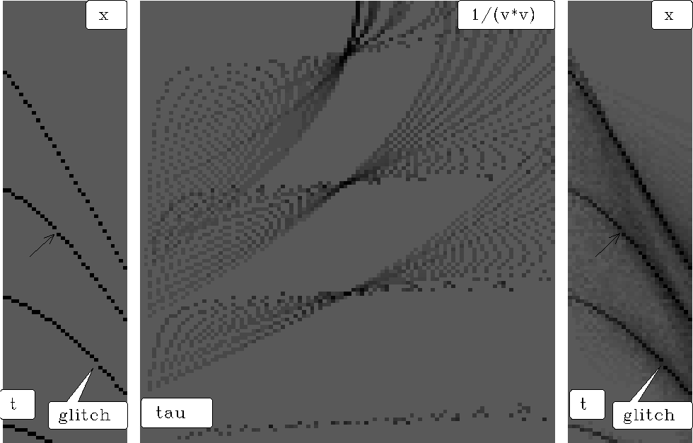
The result of the new velocity transformation is shown in Figure 3. The figure includes some scaling that will be described later.

 

vspray1
Figure 3 Offset to slowness squared and back to offset.

The code that generated Figure 3 is just like the pseudocode above except that it parameterizes velocity in uniform samples of inverse velocity squared, s=v^-2. A small advantage of using s-space instead of v-space is that the trajectories we see in $(\tau,s)$-space are readily recognized as parabolas, namely $\tau^2= t^2 - x^2 s$,where each parabola comes from a particular point in (t,x).

To exhibit all the artifacts as clearly as possible, I changed all signal values to their signed square roots before plotting brightness. This has the effect of making the plots look noisier than they really are. I also chose $\Delta t$ to be unrealistically large to enable you to see each point. The synthetic input data was made with nearest-neighbor NMO. Notice that resulting timing irregularities in the input are also present in the reconstruction. This shows a remarkable precision.

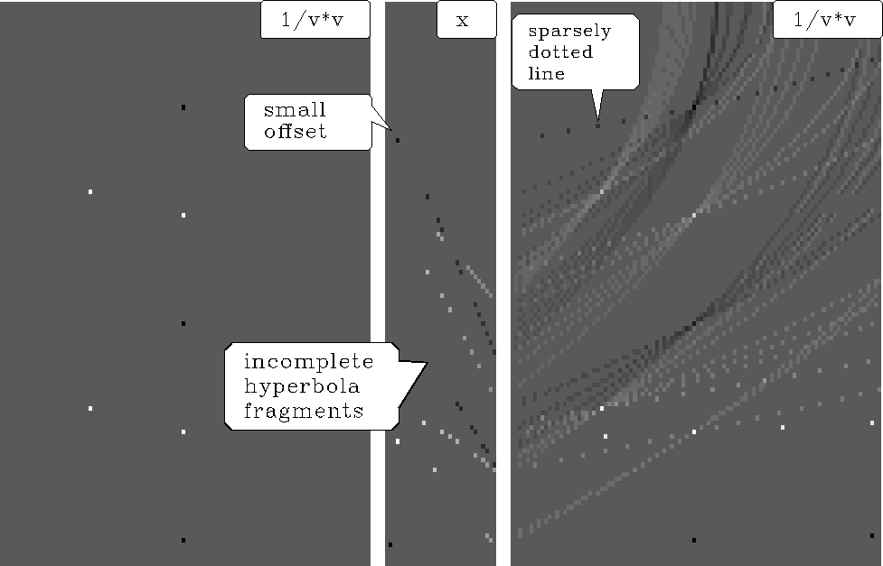
Balancing the pleasing result of Figure 3 is the poor result from the same program shown in Figure 4. The new figure shows that points in velocity space map to bits of hyperbolas in offset space--not to entire hyperbolas. It also shows that small-offset points become sparsely dotted lines in velocity space.

 

vspray2
Figure 4 Slowness squared to offset and back to slowness squared.

The problem of hyperbolas being present only discontinuously is solvable by smearing over any axis, t, x, $\tau$, or v, but we would prefer intelligent smoothing over the appropriate axis.