GEOESTIMATION: EMPTY BIN EXAMPLE

The basic formulation of a geophysical estimation problem consists of setting up two goals, one for data fitting, and the other for model smoothing. We have data $\bold d$,a map or model $\bold m$,a transformation $\bold L$,and a roughening filter $\bold A$,like the gradient $\nabla$ or the helix derivative $\bold H$.The two goals may be written as:

$$\begin{eqnarray} \bold 0 &\approx& \bold r \quad = \quad\bold L \bold m - \bold d \\ \bold 0 &\approx& \bold x \quad = \quad\bold A \bold m\end{eqnarray}$$ (13) (14)

which defines two residuals, a data residual $\bold r$,and a model residual $\bold x$, which are usually minimized by iterative conjugate-gradient, least-squares methods. A common case is ``minimum wiggliness'' when $\bold A$ is taken to be the gradient operator. The gradient is not invertable so we cannot precondition with its inverse. On the other hand, since $-\nabla^2 = \bf div \cdot grad = H'H$,taking $\bold A$ to be the helix derivative $\bold H$,we can invert $\bold A$ and proceed with the preconditioning: We change the free variable in the fitting goals from $\bold m$ to $\bold x$(by inverting (14)) with $\bold m = \bold A^{-1} \bold x$and substituting into both goals getting new goals

$$\begin{eqnarray} \bold 0 &\approx& \bold L \bold A^{-1} \bold x - \bold d \\ \bold 0 &\approx& \bold x\end{eqnarray}$$ (15) (16)

In my experience, iterative solvers find convergence much more quickly when the free variable is the roughened map $\bold x$rather than the map $\bold m$ itself.

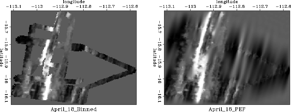
Figure 7 (left) shows ocean depth measured by a Seabeam apparatus.

 

seapef
Figure 7 Filling empty bins with a prediction-error filter.

Locations not surveyed are evident as the homogeneous gray area. Using a process akin to ``blind deconvolution'' a 2-D prediction error filter $\bold A$ is found. Then missing data values are estimated and shown on the right. Preconditioning with the helix speeded this estimation by a factor of about 30. The figure required a few seconds of calculation for about 10⁵ unknowns.

Here is how I came to the helix: For estimation theory to be practical in reflection seismology, I felt I needed a faster solution to simple problems like the Seabeam empty-bin problem. To test the idea of a preconditioner using two-dimensional polynomial division, I first coded it with the ``1.0'' in the corner. Then when I tried to put the ``1.0'' on the side where it belongs (see (6)), I could not adequately initialize the filter at the boundaries until I came upon the idea of the helix. I had never set out to solve the problem of stability of multidimensional feedback filtering (which I believed to be impossibly difficult). Serendipity.

This example suggests that the philosophy of image creation by optimization has a dual orthonormality: First, Gauss (and common sense) tells us that the data residuals should be roughly equal in size. Likewise in Fourier space they should be roughly equal in size, which means they should be roughly white, i.e. orthonormal. (I use the word ``orthonormal'' because white means the autocorrelation is an impulse, which means the signal is statistically orthogonal to shifted versions of itself.) Second, to speed convergence of iterative methods, we need a whiteness, another orthonormality, in the solution. The map image, the physical function that we seek, might not be itself white, so we should solve first for another variable, the whitened map image, and as a final step, transform it to the ``natural colored'' map.

Often geophysicists create a preconditioning matrix $\bold B$by inventing columns that ``look like'' the solutions that they seek. Then the space $\bold x$ has many fewer components than the space of $\bold m$.This approach is touted as a way of introducing geological and geophysical prior information into the solution. Indeed, it strongly imposes the form of the solution. This approach is more like ``curve fitting'' than ``inversion.'' My preferred approach is not to invent the columns of the preconditioning matrix, but to estimate the prediction-error filter of the model and use its inverse.