Wave-Equation Migration Velocity Analysis (MVA)
Estimating migration velocity by
Migration Velocity Analysis (MVA)
under complex overburden can be challenging because of
rays' inherent limitations when modeling finite-frequency
wave propagation, and because of practical problems related to
multipathing
and
poor illumination
.
The estimation of velocity under salt bodies with complex
geometry, like a rugose top,
is an important situation where conventional MVA often fails.
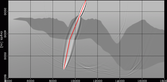
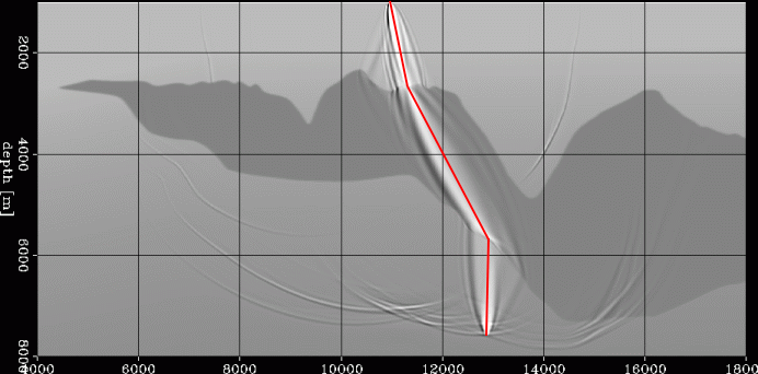
The two figures below demonstrate the inadequacy of raytracing
in modeling wave propagation through a complex salt body.
The red lines represent the geometrical ray connecting a point at the surface
to a point in the subsalt.
The ellipsoidal shapes show the finite-frequency wavepaths connecting
the same two points.
In the image on the left the wavepath can be fairly well approximated
by a fat ray because the wave propagates through a
relatively smooth part of the salt surface.
In contrast, the wavepath shown in the image on the right is too complex
to be accurately represented by the geometrical ray, or even a fat ray,
because the wavepath propagates through a rough part of the salt top.
The undulations on the top of the salt have wavelengths similar to the
wavelengths of the seismic signal, creating the complex diffraction pattern
shown in the figure.
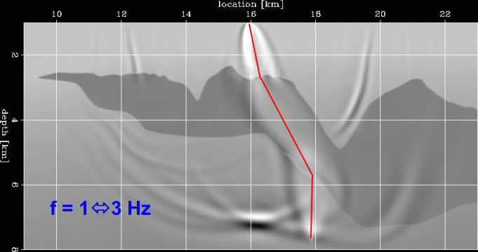
Furthermore the wavepath are inherently function of frequency,
a property that a single geometrical ray computed assuming infinite bandwidth
cannot emulate.
The figure on the right shows the frequency dependency of the wavepaths.
It shows several wavepaths with increasing bandwidth,
starting from 1-3 Hz and ending with 1-26 Hz.
As the frequency bandwidth increases,
the wavepaths narrow uniformly.
On the other hand, the diffraction patterns related to the interaction
of the wavefield with the rough top of salt
change rapidly and unpredictably with frequency.
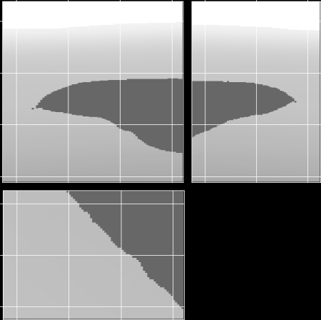
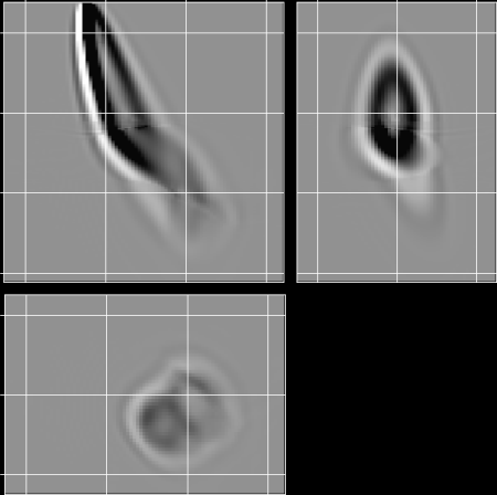
In 3-D, the wavepaths become even more complex
and more dissimilar from a simple geometrical ray.
The figure on the left show three orthogonal sections cut
through a velocity model that includes a salt edge.
The figure on the right displays the corresponding sections
cut through a wavepath for a wavefield propagating through the
salt body.
All the sections through the wavepath show that the amplitudes of the wavepath are low
around the center, where the geometrical ray would be positioned.
Furthermore,
the depth slice (bottom left) shows that the wavepath bifurcates.
To overcome the limitations of ray-based MVA
we have been developing Wave Equation MVA (WEMVA)
(
Sava, 2004
,
Sava and Biondi, 2004a
,
Sava and Biondi, 2004b
,
Chapter 11
in
3-D Seismic Imaging
).
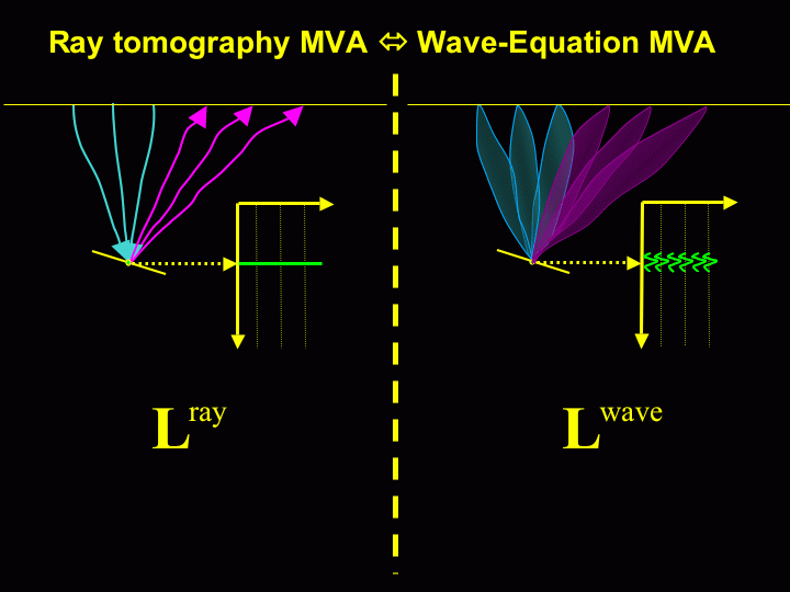
WEMVA is based on the same principle as
conventional MVA
;
that is,
to iteratively improve the flatness of ADCIG after migration by a ``tomographic''
velocity updating.
However, WEMVA performs the velocity updating using a wave-equation operator
instead of a ray-based operator.
The sketch on the left illustrates this idea.
On the left, a velocity anomaly delays propagation and
creates a perturbation in migrated ADCIGs.
In ray-based MVA we measure the depth perturbations
&Delta z
in the ADCIGs and convert them into a velocity
perturbation by inverting a ray-based linear operator.
In WEMVA (right) we extract the image perturbations
&Delta I
(whole wavefield, not simple depth shift)
and then converted them into a velocity
perturbation by inverting a wave-equation linear operator.
This operator is derived from the linearization of wave-propagation
with respect to velocity perturbations obtained by applying
the Born approximation.
To avoid that the use of the Born approximation limits the
applicability of the method to only small velocity
perturbations, we compute the image perturbation
with an appropriate differential migration operator
that makes it compliant with the Born linearization
requirements
(
Sava and Biondi, 2004a
).
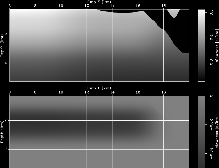
The two movies below show the application of WEMVA to a synthetic
data set modeled through the complex salt body displayed in the figures
shown at the top of this page.
The movie on the left shows four velocity fields;
the first frame shows the background velocity on the top,
and the inserted anomaly on the bottom.
The second frame shows the ``true'' anomaly on the top,
and the anomaly estimated after two non-linear iterations of WEMVA.
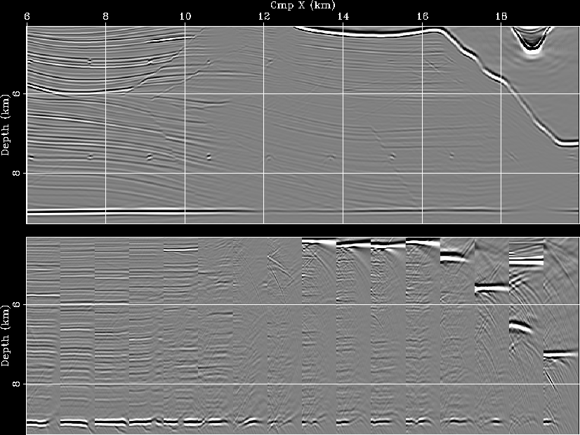
The movie on the right shows three stacked images on the top
and three sets of ADCIG corresponding to the images above;
the ADCIGs are extracted at a regular distance across the horizontal axis.
The first frame shows the migration results with the correct velocity,
the second frame shows the results with the initial velocity,
and the third frame shows the results with the estimated velocity.
The image greatly improves after the WEMVA updating and the
ADCIGs become fairly flat and similar to the ADCIGs computed
using the correct velocity.
Notice that even the ADCIGs computed with the correct velocity
are affected by artifacts caused by the poor illumination.
These illumination artifacts further complicate the velocity
estimation task under salt because they make some of the ADCIGs
unsuitable for velocity.
Sometime poorly illuminated gathers may even mislead
the inversion by creating apparent velocity errors (non flatness of events
in ADCIGs) when there are none.