Migration Velocity Analysis (MVA)

Migration needs an accurate velocity model to fully focus reflections and correctly position reflectors in space. The determination of an accurate migration velocity is a crucial step in seismic imaging. Geological knowledge of the subsurface may provide some information on the spatial distribution of propagation velocities, but detailed information can only retrieved from the seismic data themselves. Velocity estimation is based on the redundant illumination of reflectors that is provided by multi-offset seismic data. The fundamental principle underlying velocity estimation methods is that the correct velocity must accurately explain the relative time delays between reflections that are originated from the same interface in the subsurface, but were reflected with different aperture angles at the reflection point.

The large majority of velocity estimation methods are based on the analysis of the kinematic of reflections. The kinematics are analyzed directly in the data domain when both the geological structure and the velocity model are simple. A standard procedure in these cases is to measure the relative moveout of reflections as a function of offsets by computing velocity spectra. Velocity spectra are computed by applying the Normal Moveout (NMO) transformation for many trial velocities and by estimating the coherency across offsets of the NMO-transformed data by applying the semblance criterion. When either the reflector geometry is complex, or the wavefronts are distorted by a rapidly varying velocity function, the analysis of the kinematics is more robustly performed in the image domain after migration than in the data domain before migration (Chapter 10 in 3-D Seismic Imaging presents data-domain velocity estimation methods, whereas Chapter 11 presents the migrated domain velocity estimation).

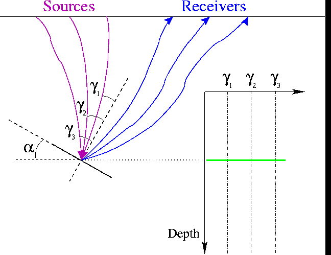
Migration Velocity Analysis (MVA) is the process of estimating interval velocity in the image domain by performing several iterations of the following three-steps process: 1) the data are migrated with the current best estimate of interval velocity, 2) the prestack images are analyzed for kinematic errors, 3) the measured kinematic errors are inverted into interval velocity updates by a tomographic process. To extract information on the velocity error, MVA exploits data redundancy in Common Image Gathers (CIG) by measuring coherency across images obtained for different data offsets, or for different reflection-aperture angles. The two movies shown below illustrate the principle of this analysis applied to Angle Domain CIGs (ADCIG) obtained by wave-equation migration .

Schematic relating velocity errors to moveout in ADCIGs.

Effects of a low velocity anomaly on the image and an ADCIG.

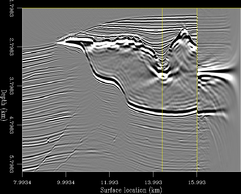
The movie on the left graphically illustrates the effects on an ADCIG caused by the addition of a low-velocity layer to the correct velocity model. The introduction of the low-velocity layer causes the image of all events (red line) to be shallower than the correct image (green line). The wide-angle events are affected more than the narrow-angle events because their path through the low-velocity layer is longer; consequently, the events smiles upward in the ADCIG. The movie on the right shows this principle in action. An erroneous low-velocity anomaly is added to the correct velocity model in the canyon on the top of the salt. The ADCIG at the bottom of the canyon smiles upward because all the angles are affected by the anomaly. In contrast, only the narrow-angle events in the ADCIG below the salt are pulled upward, whereas the far-angle events are unaffected by the introduction of the anomaly.

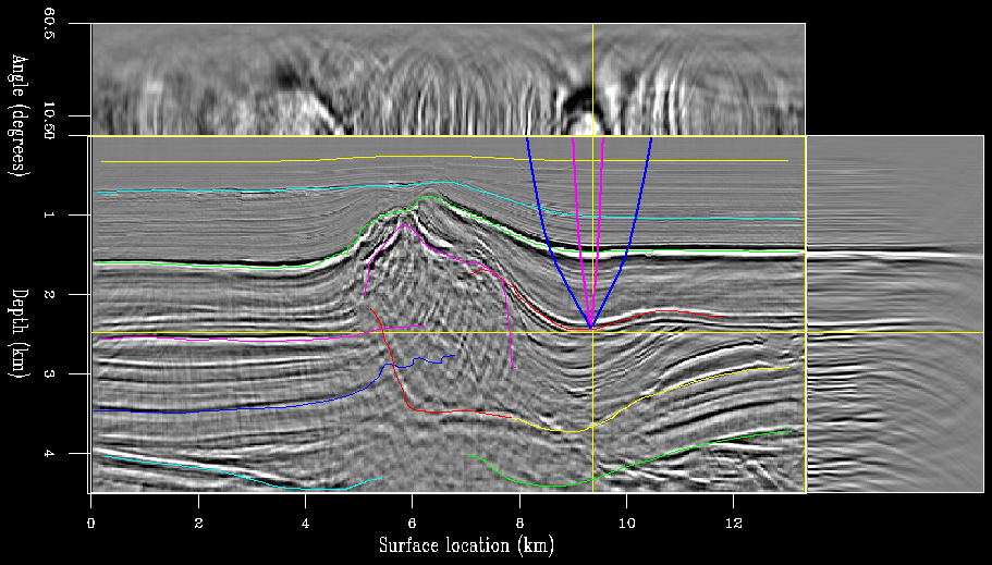
Graphic illustration of the MVA process from ADCIGs obtained by wave-equation migration.

The deviation from flatness measured in the migrated ADCIGs can be quantitatively related to kinematic errors accumulated by the wave propagation through an inaccurate migration-velocity model ( Biondi and Symes, 2004 ; Biondi and Tisserant, 2004 ), and the kinematic errors can be inverted in velocity errors by a tomographic method. The figure on the right graphically illustrates this inversion procedure. The strongest reflectors are picked in the stacked image (left panel) and the the events corresponding to these reflectors in the ADCIGs (right panel) are analyzed for departure from flatness, usually by applying some kind of Residual Moveout (RMO) analysis. The RMO analysis provides measurements of depth errors that are then transformed into traveltime perturbations. These traveltime perturbations are inverted into velocity perturbations by a ray-based tomographic inversion based on a large collection of rays traced from the surface to the reflectors, as the ray represented by the blue ad magenta lines superimposed onto the image. This process is repeated several times in order to converge to a satisfactory result.

The tomographic inversion problem is largely undetermined. The ray coverage has a limited angular range because the most of the rays are close to be vertical. The inversion process must be thus constrained to avoid the solution to diverge. Geological knowledge on the subsurface structures and on the behavior of the velocity function should be used to constraints the components of the velocity model that are not sufficiently determined from the data alone. The constraint are usually applied by introducing a regularization term into the objective function to be minimized. Conventional regularization methods steer the solution toward a model that is along all the spatial directions. However, an isotropic smoother, such as a Laplacian regularization term, does not take advantage of our knowledge that in many geological settings velocity tends to be smooth within a layer, but may have discontinuities at the boundaries between layers. This geological knowledge can be incorporated by designing a regularization term that privileges a velocity function that is smoother in the direction parallel to the reflectors than in the direction orthogonal to the reflectors ( Clapp, 2000 ; Clapp et al., 2004 ).

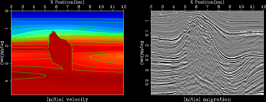
The movie below compares the results obtained by a tomographic MVA method that uses a conventional isotropic smoother in the depth domain (labeled Depth-Laplacian in the movie), with a tomographic MVA method that uses a layer-oriented smoothing in the Tau domain (labeled Tau-Steering in the movie). The panels on the left show the velocity model, whereas the panels on the right show the corresponding migrated image. In both cases the tomographic MVA converges to a velocity model that is a substantial improvement over the initial velocity model and the initial migrated image. The result of the structural regularization applied in the tau domain provides a more geologically plausible velocity model, that yields a better focused migrated image.

Comparison of MVA results using conventional MVA and MVA in tau domain with structural regularization.