| Model | In-line dip ( |
X-line dip ( |
Layer Velocity (km/s) |
| A | (0.0,5.0,10.0) | (0.0, 0.0, 0.0) | (1.5, 2.0, 2.5) |
| B | (0.0,5.0,10.0) | (0.0, -5.0, 5.0) | (1.5, 2.0, 2.5) |
Combining the multiple prediction and the PSMCG interpolation, we get a new, practical multiple prediction scheme beyond two dimension. In this section, two 3-D synthetic datasets with similar acquisition geometries are used to evaluate the performance of the new scheme. The corresponding model and acquisition parameters are given in Tables 1 and 2.
| Model | In-line dip ( |
X-line dip ( |
Layer Velocity (km/s) |
| A | (0.0,5.0,10.0) | (0.0, 0.0, 0.0) | (1.5, 2.0, 2.5) |
| B | (0.0,5.0,10.0) | (0.0, -5.0, 5.0) | (1.5, 2.0, 2.5) |
| Model | |||
| A | 20 | 20 | 100 |
| B | 20 | 20 | 50 |
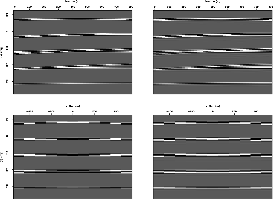
Model A is designed so that the shotline and streamers are deployed along the in-line dip direction. Therefore, there is no approximation error in our approach. With 11 streamers covering from -500m to +500m and 100m streamer interval in the cross-line direction, this is a wide azimuth survey. For a given shot location, the ideal multiple gather and the predicted one are shown in Figure 8. Each 3-D MCG cube in this example is first stacked along the in-line direction into a 2-D PSMCG containing at most 11 traces of 100m sampling interval. The 2-D PSMCG is then interpolated in the cross-line direction to be sampled at 25m interval. The interpolated PSMCG is further stacked into a trace.
|
wa2d-mult
Figure 8 In-line dip model. Left: ideal multiple reflection. Right: estimated multiple reflection. |  |
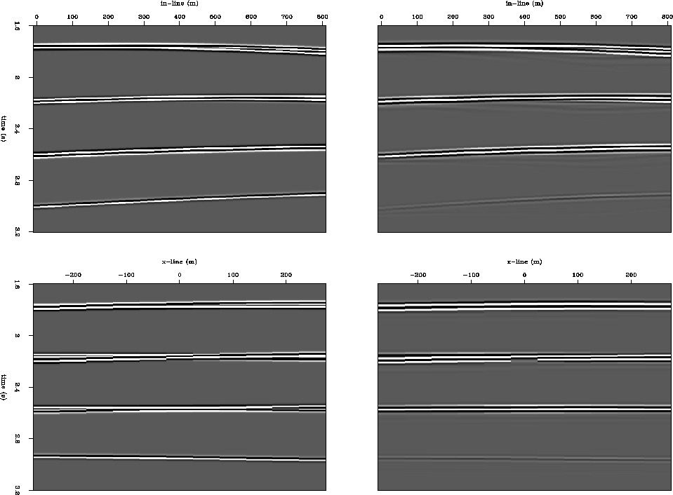
Model B is a relatively narrow azimuth survey with still 11 streamers covering from -250m to +250m and 50m streamer interval in the cross-line direction. The bottom two reflectors in the model have the opposite cross-line angles, which, inevitably, introduce the approximation error in the estimation. However, as shown in Figure 9, as long as the cross-line dips have no dominant direction, the error is usually tolerable and can possibly be handled in the subtraction step.
|
na3d-mult
Figure 9 Mixing dip model. Left: ideal multiple reflection. Right: estimated multiple reflection. |  |