

Next: CONCLUSIONS
Up: Velocity estimation: Clapp, et
Previous: ADDITIONAL CONCERNS
An attractive feature of the velocity-estimation
procedure defined in this paper is that it is linear.
This means there should be no unpleasant surprises
associated with multiple minima
or with convergence speed.
If bad results are found, they should arise directly
from bad RMS velocity picks or from
the possibly inappropriate association of
stack power with the statistical weighing function.
Another attractive feature of the velocity-estimation procedure defined here
is that it leads directly to a rational approach
to finding interval velocity as a function of midpoint.
Traditionally, velocity at each midpoint is estimated separately.
Thus one midpoint cannot help neighboring estimates,
nor are unrealistically rapid variations
with midpoint suppressed in a natural way.
For example, suppose we redefine our fitting goals as:
| ![\begin{eqnarray}
0 &\approx& \bold W'
\left[
\bold C^2 \bold L^{-1} \bold p
-
\bold d
\right]
\ \bold 0
&\approx&
\epsilon \bold p .\end{eqnarray}](img22.gif) |
(10) |
| (11) |
where  is a roughening operator such as the
Laplacian
(in the space of midpoint and traveltime depth)
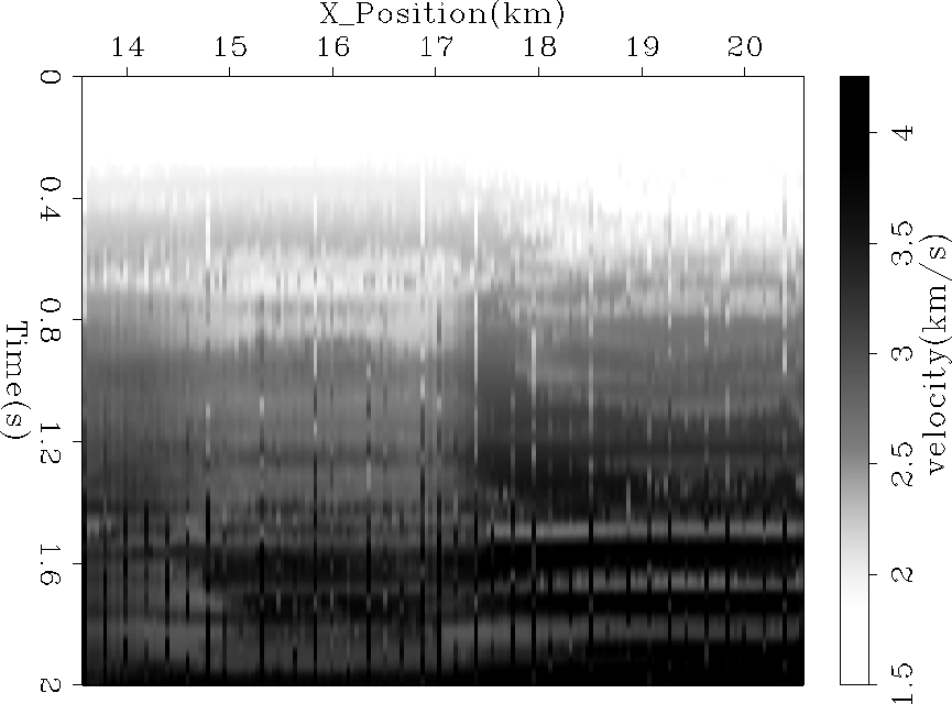
Starting with picked RMS velocities (Figure data2d) from
a North Sea salt structure,
attempted to invert for interval velocity.
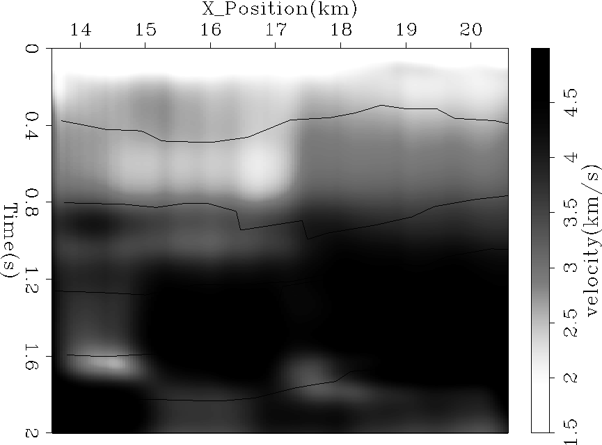
As Figure vint2d shows, for small, long wavelength
variations in lateral velocity (Dix being approximately correct) we obtain
a smooth, reasonable interval velocity model with minimal effort.
data2d
Figure 10 2-D RMS velocity function picked
by finding the maximum semblance within a fairway. Note that for some CMP
locations, the picked velocity is completely inaccurate. The inversion algorithm
takes these inaccuracies into account and leads to a smooth model (vint2d).


 vint2d
Figure 11 2-D interval velocity function
obtained from applying fitting goals (10) and
(11) after 30 iterations.


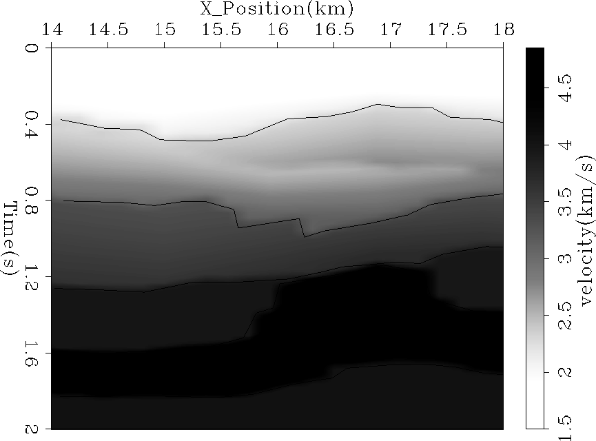
For a further test we replaced the Laplacian of
equation (11) with steering filters
Clapp et al. (1997) built from dips off an interval
interval velocity model
(Figure ![[*]](http://sepwww.stanford.edu/latex2html/cross_ref_motif.gif) ) built with a more sophisticated
scheme (nearest offset section could just have easily been used).
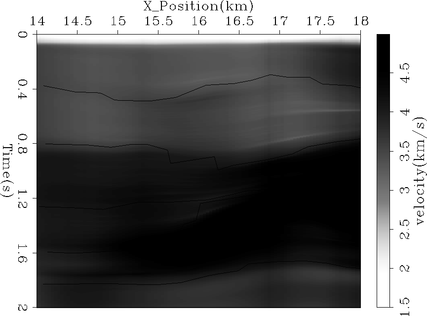
We then applied
the 2-D inversion and obtained Figure
) built with a more sophisticated
scheme (nearest offset section could just have easily been used).
We then applied
the 2-D inversion and obtained Figure ![[*]](http://sepwww.stanford.edu/latex2html/cross_ref_motif.gif) . Generally,
we did a good job recovering the salt structure, but are still susceptible
to multiple infected velocity picks.
. Generally,
we did a good job recovering the salt structure, but are still susceptible
to multiple infected velocity picks.
reflectors-cor
Figure 12 Supplied interval velocity
model with picked reflectors superimposed.


 reflectors-est
Figure 13 Estimated interval velocity
model with picked reflectors superimposed.


Next: CONCLUSIONS
Up: Velocity estimation: Clapp, et
Previous: ADDITIONAL CONCERNS
Stanford Exploration Project
7/6/1998


![[*]](http://sepwww.stanford.edu/latex2html/cross_ref_motif.gif) ) built with a more sophisticated
scheme (nearest offset section could just have easily been used).
We then applied
the 2-D inversion and obtained Figure
) built with a more sophisticated
scheme (nearest offset section could just have easily been used).
We then applied
the 2-D inversion and obtained Figure ![[*]](http://sepwww.stanford.edu/latex2html/cross_ref_motif.gif) . Generally,
we did a good job recovering the salt structure, but are still susceptible
to multiple infected velocity picks.
. Generally,
we did a good job recovering the salt structure, but are still susceptible
to multiple infected velocity picks.

