


| |
(9) | |
![[*]](http://sepwww.stanford.edu/latex2html/cross_ref_motif.gif) shows, our velocity function is
approximately linear within
the layers and has a reduced wiggliness compared to the smooth interval velocity curve.
shows, our velocity function is
approximately linear within
the layers and has a reduced wiggliness compared to the smooth interval velocity curve.
|
bvint.stack
Figure 4 The result of the inversion for a blocky velocity model using the fitting goals (9). | 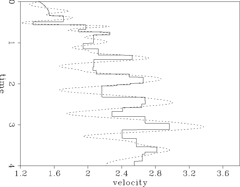 |


 |