


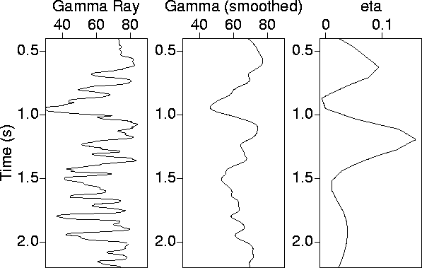
To verify the preceding observations, Figure 9
and 10
compares the ![]() curves with gamma
ray logs available from nearby wells. Two locations are shown, one at
CMP 1100,
another, close by, at CMP 1220. At both locations, the Gamma ray logs indicate
the presence of sands just prior to the one second mark. At this time, the
curves with gamma
ray logs available from nearby wells. Two locations are shown, one at
CMP 1100,
another, close by, at CMP 1220. At both locations, the Gamma ray logs indicate
the presence of sands just prior to the one second mark. At this time, the ![]() curve also
shows small values suggesting the this part of the vertical column is isotropic.
Because shales induce anisotropy, more likely than not, this part of the section
corresponds to sands. Figure 6 provides information from seismic data of the
lateral extent of this sand layer, or layers. At CMP locations 1100 and 1220,
the correlation between
the well-log measurements, at a lower resolution,
and the
curve also
shows small values suggesting the this part of the vertical column is isotropic.
Because shales induce anisotropy, more likely than not, this part of the section
corresponds to sands. Figure 6 provides information from seismic data of the
lateral extent of this sand layer, or layers. At CMP locations 1100 and 1220,
the correlation between
the well-log measurements, at a lower resolution,
and the ![]() curve is remarkable. Recall, that the
curve is remarkable. Recall, that the ![]() curve is obtained in its entirety from P-wave surface seismic data. Yet, information
like the low frequency
character of the shale-sand content is extracted from these data.
curve is obtained in its entirety from P-wave surface seismic data. Yet, information
like the low frequency
character of the shale-sand content is extracted from these data.
 |

 |