Constructing an ``isotropic'' Laplacian operator

The problem of approximating the Laplacian operator in two dimensions not only inherits the inaccuracies of the one-dimensional finite-difference approximations, but also raises the issue of azimuthal asymmetry. For example, the usual five-point filter  

$$F_5 = \begin{array} {\vert r\vert r\vert r\vert} \hline 0 & ... ... \hline 1 & -4 & 1 \\ \hline 0 & 1 & 0 \\ \hline \end{array}$$ (26)

exhibits a clear difference between the grid directions and the directions at a 45-degree angle to the grid. To overcome this unpleasant anisotropy, we can consider a slightly larger filter of the form  

$$F_9 = \begin{array} {\vert r\vert r\vert r\vert} \hline \alp... ...amma \\ \hline \alpha & \gamma & \alpha \\ \hline \end{array}$$ (27)

where the constants $\alpha$ and $\gamma$ are to be defined. The Fourier-domain representation of filter (27) is  

$$F_9 (k_x,k_y) = 4\,\alpha\,[\cos{k_x}\,\cos{k_y} - 1] + 2\,\gamma\,[\cos{k_x}+\cos{k_y}-2]\;,$$ (28)

and the isotropic filter that we can try to approximate is defined analogously to its one-dimensional equivalent, as follows:  

$$F (k_x,k_y) = 2 (\cos{k} -1) = 2 (\cos{\sqrt{k_x^2+k_y^2}} - 1)\;.$$ (29)

Comparing equations (28) and (29), we notice that they match exactly, when either of the wavenumbers k_x or k_y is equal to zero, provided that  

$$\alpha = \frac{1-\gamma}{2}\;.$$ (30)

Therefore, we can reduce the problem to estimating a single coefficient $\gamma$. Another way of expressing this conclusion is to represent filter F₉ in equation (28) as a linear combination of filter F₅ from equation (28) and its rotated version Cole (1994), as follows:  

$$F_9 = \gamma\, \begin{array} {\vert r\vert r\vert r\vert} \... ...line 0 & -2 & 0 \\ \hline 1/2 & 0 & 1/2 \\ \hline \end{array}$$ (31)

With the value of $\gamma=0.5$, filter F₉ takes the value  

$$F_9 = \begin{array} {\vert r\vert r\vert r\vert} \hline 1/4 ... .../2 & -3 & 1/2 \\ \hline 1/4 & 1/2 & 1/4 \\ \hline \end{array}$$ (32)

and corresponds precisely to the nine-point McClellan filter Hale (1991a); McClellan (1973). On the other hand, the value of $\gamma=2/3$ gives the least error in the vicinity of the zero wavenumber k. In this case, the filter is  

$$F_9 = \begin{array} {\vert r\vert r\vert r\vert} \hline 1/6 ... ...& -10/3 & 2/3 \\ \hline 1/6 & 2/3 & 1/6 \\ \hline \end{array}$$ (33)

Errors of different approximations are plotted in Figure 11

 

laplace
Figure 11 The numerical anisotropy error of different Laplacian approximations. Both the five-point Laplacian (plot a) and its rotated version (plot b) are accurate along the axes, but exhibit significant anisotropy in between at large wavenumbers. The nine-point McClellan filter (plot c) has a reduced error, while the filter with $\gamma=2/3$ (plot d) has the flattest error around the origin.

Under the helix transform, a filter of the general form (27) becomes equivalent to a one-dimensional filter with the Z transform

   $$\begin{eqnarray} F_9 (Z) & = & \alpha\,Z^{-N_x-1} + \gamma\,Z^{-N_x} + \alpha\,Z... ...ma\,Z + \alpha\,Z^{N_x-1} + \gamma\,Z^{N_x} + \alpha\,Z^{N_x+1}\;,\end{eqnarray}$$

where N_x is the helix period (the number of grid points in the x dimension). To find the inverse of a convolution with filter (34), we factorize the filter into the causal minimum-phase component and its adjoint:  

$$F_9 (Z) = P (Z) P (1/Z)\;.$$ (35)

To find the coefficients of the filter P, any one-dimensional spectral factorization method can be applied. It is important to point out that the result of factorization (neglecting the numerical errors) does not depend on N_x. Another approach is to define a residual error vector for the coefficients of Z in equation (35) and minimize it for some particular norm. For example, minimizing the $\mathcal{L}_1$ norm when F₉ is the McClellan filter (32), we discover that the filter P, after transforming back to two dimensions, takes the form  

$$\begin{array} {\vert r\vert r\vert r\vert r\vert r\vert r\ve... ...3 & 0.0808 & 0.2543 & 0.3521 & 0.1553 & & \\ \hline\end{array}$$ (36)

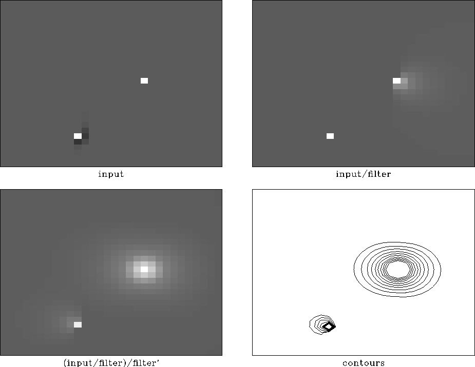
The results of applying a recursive deconvolution with filter (36) are shown in Figure 12. An essentially similar procedure, only with a different set of filters, works for implicit wavefield extrapolation.

 

inv-laplace
Figure 12 Inverting the Laplacian operator by a helix deconvolution. The top left plot shows the input, which contains a single spike and the causal minimum-phase filter P. The top right plot is the result of inverse filtering. As expected, the filter is deconvolved into a spike, and the spike turns into a smooth one-sided impulse. After the second run, in the backward (adjoint) direction, we obtain a numerical solution of Laplace's equation! In the two bottom plots, the solution is shown with grayscale and contours.