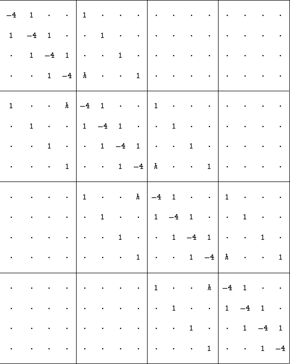
 |
(5) |
The two-dimensional matrix of coefficients for the Laplacian operator
is shown in (5),
where,
on a cartesian space, h=0,
and in the helix geometry, h=1.
(A similar partitioned matrix arises from packing
a cylindrical surface into a ![]() array.)
Notice that the partitioning becomes transparent for the helix, h=1.
array.)
Notice that the partitioning becomes transparent for the helix, h=1.
With the partitioning thus invisible, the matrix simply represents one-dimensional convolution and we have an alternative analytical approach, Fourier Transform. We often need to solve sets of simultaneous equations with a matrix similar to (5). A costly method is to factor the matrix into upper and lower triangular form that can be ``backsolved'' which in this case amounts to recursive filtering.
The Fourier approach is similar but much faster.
The (negative of the) Laplacian operator is regarded as an
autocorrelation ![]() .Using the Kolmogoroff spectral-factorization method,
a ``minimum-phase'' wavelet is found which has this autocorrelation.
This 2-D wavelet (rotated
.Using the Kolmogoroff spectral-factorization method,
a ``minimum-phase'' wavelet is found which has this autocorrelation.
This 2-D wavelet (rotated ![]() from (4)) is
from (4)) is
| |
(6) |
 |
As a practical matter, this Poisson equation solver is a convenient isotropic smoothing filter.
Twenty years ago when migrations were two-dimensional,
we developed powerful wave-equation methods
for finite-difference downward-continuation of wave fields.
These methods were frustrated in 3-D
because we could not rapidly solve algebraic systems like
![]() .The helix should resuscitate these methods
(although we will need to develop approximations
for when
.The helix should resuscitate these methods
(although we will need to develop approximations
for when ![]() ).
).