


Next: About this document ...
Up: Alkhalifah and Fomel: Anisotropy
Previous: Relating the zero-offset and
Although the exact expressions might be sufficiently constructive for
actual residual migration applications, linearized forms are still
useful, because they give us valuable insights into the problem. The
degree of parameter dependency for different reflector dips is one of
the most obvious insights in the anisotropy continuation problem.
Perturbation of a small parameter provides a general mechanism to
simplify functions by recasting them into power-series expansion over
a parameter that has small values. Two variables can satisfy the small
perturbation criterion in this problem: The anisotropy parameter
 (
( ) and the reflection dip
  (
( or px v <<1).
Setting  yields equation (19) for the velocity continuation
in elliptical anisotropic media and
yields equation (19) for the velocity continuation
in elliptical anisotropic media and
|  |
(27) |
which represents the case when we initially introduce anisotropy into our model.
Because px (the zero-offset slope) is typically lower than
(the migrated slope), we perform initial expansions in
terms of y=px v. Applying the Taylor series expansion of
equations (12) and (13) in terms of y and
dropping all terms beyond the fourth power in y, we obtain
|  |
(28) |
and
|  |
(29) |
Although both equations are equal to zero for px=0, the leading
term in the velocity continuation is proportional to px2,
whereas the the leading term in the continuation is
proportional to px4. As a result the velocity continuation has
greater influence at lower angles than the continuation. It
is also interesting to note that both leading terms are independent
of the size of anisotropy ().
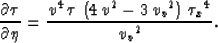
Despite the typically lower values of px, expansions in terms of
are more important, but less accurate. For small , , and, therefore, the leading-term behavior of
expansions is the same as that of px As a result, we
arrive at the equation
, and, therefore, the leading-term behavior of
expansions is the same as that of px As a result, we
arrive at the equation
|  |
(30) |
and
|  |
(31) |
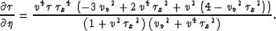
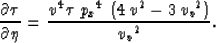
Most of the terms in equations (B-4) and (B-5) are
functions of the difference between the vertical and NMO
velocities. Therefore, for simplicity and without a loss of
generality, we set vv=v and keep only the terms up to the eighth
power in . The resultant expressions take the form
|  |
(32) |
and
|  |
(33) |
Curiously enough, the second term of the continuation
heavily depends on the size of anisotropy ( ). The first
term of equation (B-6) (
). The first
term of equation (B-6) ( ) is the isotropic
term; all other terms in equations (B-6) and (B-7)
are induced by the anisotropy.
) is the isotropic
term; all other terms in equations (B-6) and (B-7)
are induced by the anisotropy.
Next: About this document ...
Up: Alkhalifah and Fomel: Anisotropy
Previous: Relating the zero-offset and
Stanford Exploration Project
11/11/1997