Stack equalization

In his notes 3-D seismic imaging , Biondo Biondi discusses partial stacking as the simplest prototype example of an imaging operator. A simple implementation of partial stacking can employ normal moveout (NMO) to correct for traveltime differences in the data. Stacking irregular data after residual NMO can be regarded then as an inverse interpolation problem, which one can solve by optimization methods. In this section, I include a simple example of an efficient data-space regularization for optimizing partial stack.

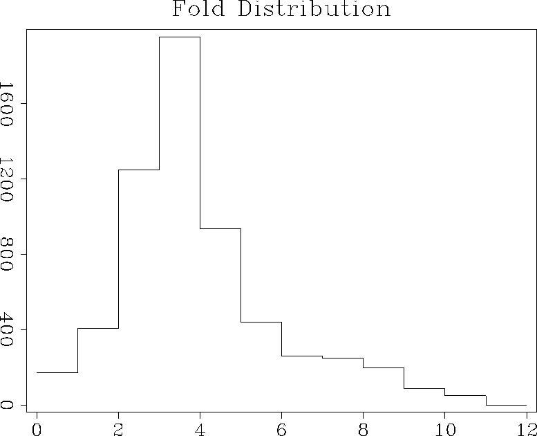
Following Biondi's reproducible example, I use a potion of the Conoco North Sea dataset with offsets, windowed in the range from 400 to 600 m. The geometry of the CMP locations of the input traces is illustrated in Figure 10. The fold distribution, shown as a map view in Figure 11 and as a histogram in Figure 12 is fairly dense overall, but has noticeable holes (empty bins). The regions of zero fold make the inverse interpolation problem underconstrained and suggest an application of a regularized optimization scheme.

 

cmp Figure 10 Midpoint geometry of the input data

 

fold Figure 11 Fold distribution of the input data. A map view.

 

hist Figure 12 Fold distribution of the input data. A histogram.

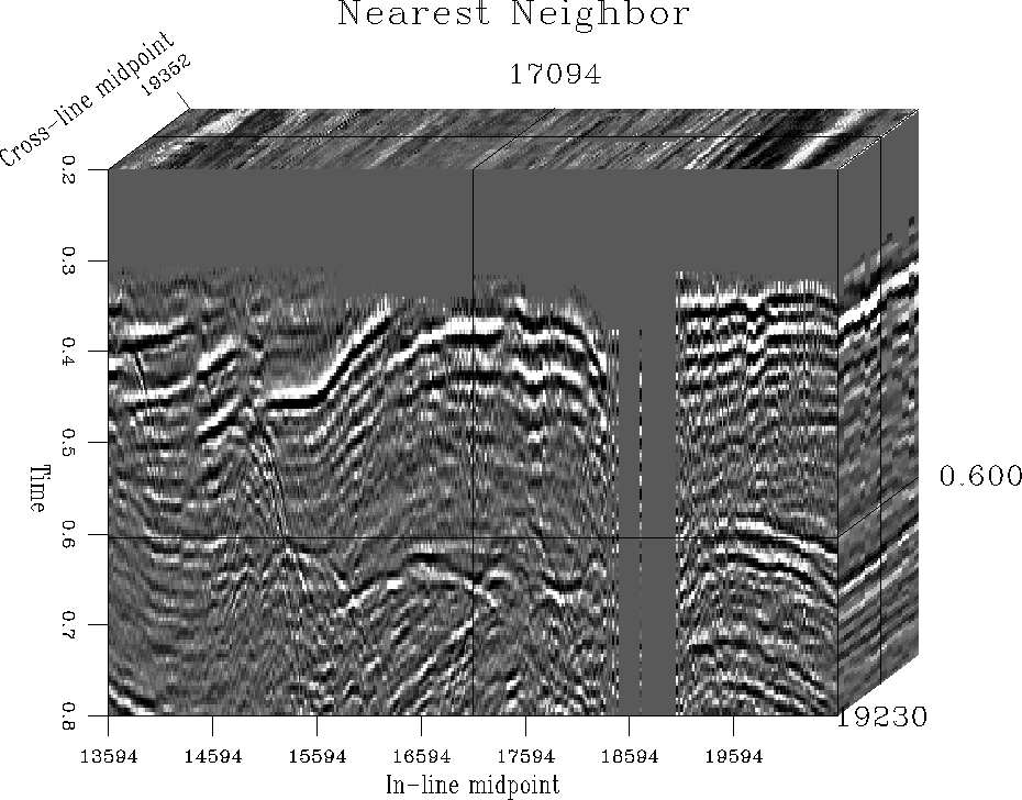
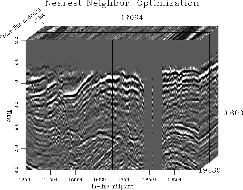
Figure 13 shows the result of simple binning (the adjoint of nearest neighbor interpolation), normalized by the inverse of the fold density. Obviously, the regions of zero fold don't receive any signal, which can lead to undesirable artifacts in future processing. Figure 14 is the result of non-regularized optimization, with 5 conjugate-gradient iterations at each time slice level. This approach not only fails to fill the empty holes, but also creates unbalanced output because of the poor conditioning of the inverse problem. Figure 15 shows the result of a data-space regularized inversion with a small smoothing filter as a preconditioner. The convergence is fast, and the result looks much improved. Because of the fast convergence of the data-space regularization, the inverse interpolation scheme is inexpensive to apply. One easy way of improving the result further is to change the simple nearest neighbor interpolation operator to a more accurate one. 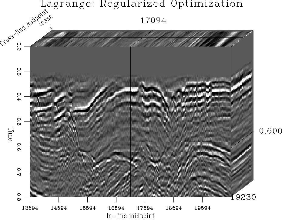Figure 16 is the result of the regularized inverse interpolation with the Lagrange 4-point interpolator.

 

bin
Figure 13 Data transformed to a regular grid by normalized adjoint interpolation (simple binning.)

 

invbin
Figure 14 Data transformed to a regular grid by non-regularized inverse interpolation.

 

regbin
Figure 15 Data transformed to a regular grid by data-space regularized inverse interpolation.

 

regtin
Figure 16 Data transformed to a regular grid by data-space regularized inverse interpolation, using Lagrange's 4-point interpolator as the forward interpolation operator.

As demonstrated by Biondi et al. (1996), an accurate interpolation for dipping reflector events and diffractions requires the azimuth moveout operator. Another interesting, though untested, approach is to use the inverse of a prediction-error filter for preconditioning the inverse interpolation.