ALIASING & COVERAGE

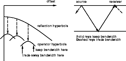
Considering the degree to which data may be aliased on the crossline offset axis, it is likely that a straightforward bandpass-type antialiasing will force unacceptable cuts in frequency content. However, antialiasing can be tuned to preserve more signal bandwidth, provided that compensating bandwidth can be traded away elsewhere. A threshold frequency for antialiasing may be calculated from:

$$\omega_{\rm threshold} = \frac{v}{4 \Delta x \sin \theta}$$ (1)

Yilmaz (1987). The $\theta$ in equation 1 is measured relative to a vertically traveling plane wave, but some other plane wave may be chosen. In poststack migration, for instance, it is reasonable to assume that data will have a wide range of positive and negative dips, so a principal dip of zero (vertical plane wave) makes sense. In the prestack datuming case, it may be that the range of time dips is limited, depending on the subset of data you are examining. A given source-receiver combination's contribution to the output space will have some optimum principle time dip, which is not necessarily zero. Considering the simple case of a flat earth, it can be seen that shot gather continuation should antialias relative to some plane wave dipping towards increasing offset. In the illustrated case, the outer offset flank of the datuming hyperbola contributes to constructing the reflection hyperbola. The inner offset flank contributes only to destructive interference with other inner offset flanks. Choosing a particular hyperbola flank is like choosing shot and receiver take-off angles. Preserving the inner offset portion of the hyperbola is like preserving energy which has divergent take offs (see Figure 1). The ray approaching the receiver from the side opposite the source makes sense in the case of a strongly dipping reflector.

 

simp-pic
Figure 1 For simple earth models, the principal dip for antialiasing purposes can be chosen to favor the increasing offset portion of the operator hyperbola.

The operator impulse response, antialiased with respect to a horizontally travelling plane wave, is shown in figure 2. Turning the plane wave horizontal is overkill, but it illustrates the principle plainly. It also illustrates an important point related to the interaction of the inline and crossline directions. Compensating for sparse sampling in the crossline direction by changing the principal dip should not interfere with the well sampled inline direction. A vertically travelling plane wave and a plane wave travelling horizontally in the crossline direction are an equal ninety degrees from a wave travelling in the inline direction.

 

imp
Figure 2 Antialiased operator impulse response.

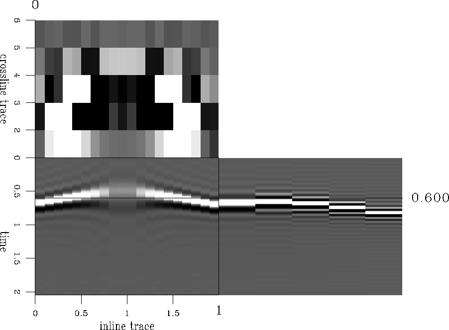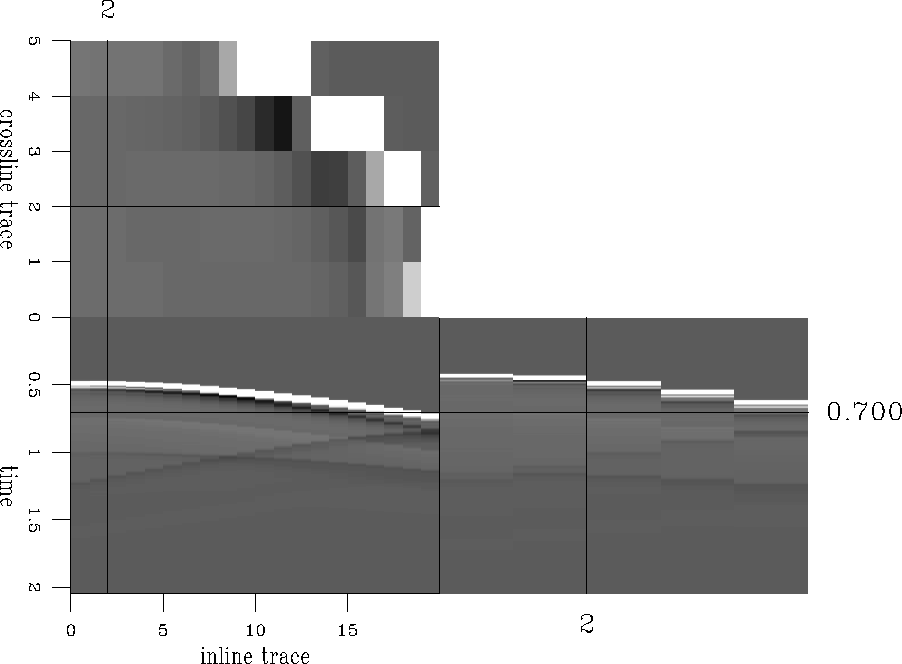
A simple 3D synthetic shot gather is shown in Figure 3. Here the crossline receiver spacing is four times the inline spacing. It is easy to see that the reflection event is mildly aliased in the inline direction, and severely aliased in the crossline. The gather is shown in Figure 4 after upward continuation. Note that there is a noticeable event other than the reflection; this is the upward continuation of a modeling artifact, visible in the original. Also note that the data still contain frequencies above the spatial nyquist.

 

synth3din
Figure 3 3D synthetic input. The crossline direction is subsampled relative to the inline.

 

synth3dout
Figure 4 The 3D synthetic after upward continuation. Some crossline bandwidth is preserved, without generation of artifacts (though a modeling artifact -the black event dipping to the left- has been exacerbated).

Conflicting dips created by negative offset (acquisition geometry) do not create a problem, because each input trace is a separate experiment and may be antialiased with a particular principle time dip, so long as that dip corresponds to an energetic part of the wavefield. However, conflicting dips in the data due to dipping reflectors in the earth do create a problem. This energy propagates through the most strongly antialiased part of the datuming hyperbola, and so will lose a great deal of energy and bandwidth.

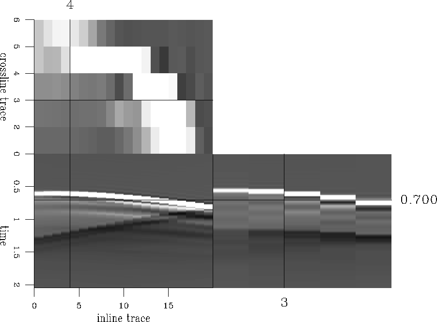
Changing to midpoint and offset coordinates allows one to safely favor positive dips. However, the operator is no longer separable along the two axes, so it is considerably more expensive to apply. Also, the optimum principle time dip becomes a relatively complicated function of input offset, output offset, midpoint dip, and time, as illustrated to some degree in Figure 5. Some optimum time must be chosen based on shot and receiver geometries.

 

comp-pic Figure 5 In midpoint and offset, the optimum principle time dip is a function of midpoint dip and offsets.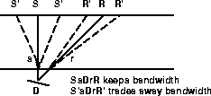