AN ITERATIVE LEAST-SQUARE INVERSION SCHEME

Our revised amplitude model is

$$a^{total}_{s,h} \; = \; a_{s} \: a_{h} \: a_{y \, = \, s \, + \, h/2} \: a_{r \, = \, s \, + \, h} \: a_{earth}$$ (1)

where a_earth is the earth low-frequency component of the amplitude function; and a_s, a_h, a_y, and a_r are the components of the amplitude caused by the source (s), the full offset (h), the midpoint (y), and the receiver (r) variations, respectively.

We now need to invert for the amplitude correction coefficients in order to remove the stripes in Figure 1. To do so, we use the following quadratic objective function

$$\varphi \; = \; \; \parallel \, d \, \left( s, h \right) \: - \: a_{s} \: a_{h} \: a_{y} \: a_{r} \, \parallel^{2}$$ (2)

where we assume that the data d can be modeled as the product of the source, offset, midpoint, and receiver. Normalization allows us to assume $a_{earth} \approx 1$.

To estimate the coefficients a_s, a_h, a_y, and a_r we choose the Gauss-Seidel algorithm which is an iterative least-square inversion scheme [see Stark 1970]. We also assume that the coefficients for which we are solving the objective function $\varphi$ are independent. Therefore, we can get an estimation of one type of coefficient (a_s, a_h, a_y, or a_r) while keeping the value of the other fixed.

Under these assumptions, after minizing the objective function with respect to the source coefficients, we derive the following expression, giving the value of the coefficients at iteration k as a function of the other coefficients at the preceding iteration:

$$a_{s}^{(k)} \: = \: \frac{\sum_{h} \; d \; a_{h}^{(k \, - \,... ... \: a_{y}^{(k \, - \, 1)} \: a_{r}^{(k \, - \, 1)} \right]^2}$$ (3)

We obtain a similar expression for the other three coefficients, where each is expressed as a function of the data and all the other coefficients.

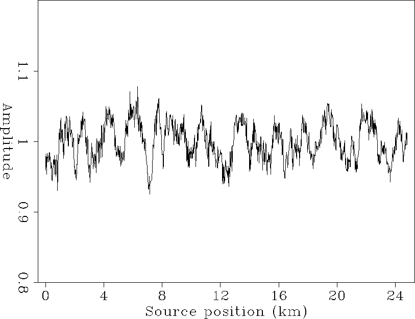
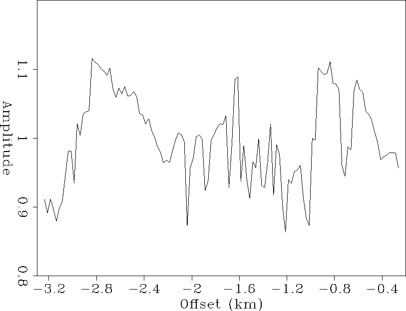
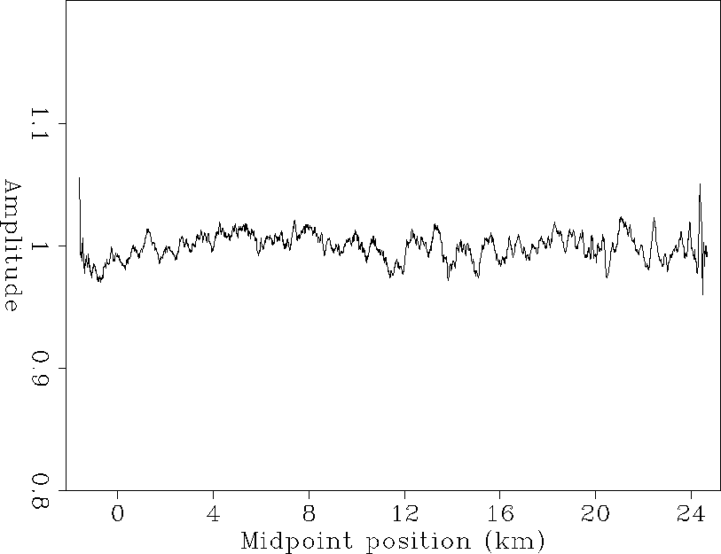
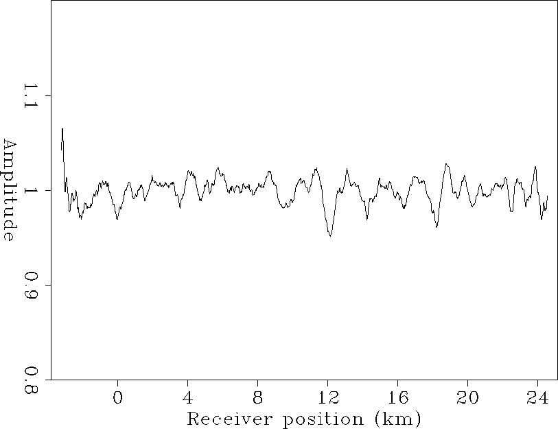
Figures 4, 5, 6, and 7 show the result of the inversion when the algorithm has converged, which required 10 iterations. Comparing the source and offset correction coefficient curves (Figures 4 and 5) with those obtained by Berlioux and Lumley 1994, we can see that the global shape of the curves is the same. The curves in Figures 4 through 7 show identical features: high-frequency variations of the coefficient value around a globally constant value.

 

source
Figure 4 Estimated source coefficients.

 

offset
Figure 5 Estimated offset coefficients.

 

midpoint
Figure 6 Estimated midpoint coefficients.

 

receiver
Figure 7 Estimated receiver coefficients.

The next section shows how we use these estimated correction coefficients to cancel the stripes in the original 2-D amplitude map, and thus balance the traces in the survey.