An example of calculating a prediction-error filter

The problem of calculating a prediction-error filter $\sv f$can be set up by describing the convolution process as a matrix multiplication $\st A \sv f$.The matrix $\st A$ is made up of shifted versions of the signal $\sv x$to be multiplied by the filter vector $\sv f$ as shown below. If $\sv x$ is perfectly predictable, a filter $\sv f$ will be calculated to give a result of zero, $\st A\sv f=\sv 0$. With most real data, $\sv x$ will not be perfectly predictable, and the result of $\st A \sv f$ will not be zero, but $\st A \sv f = \sv r$,where $\sv r$ is the error or unpredictable part. This error is minimized to get the desired $\sv f$.The idea of an imperfect prediction may also be expressed as a system of regressions, where $\st A\sv f \approx \sv 0$.

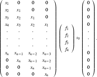
Here, I will show the traditional method of setting up a one-dimensional prediction-error filter calculation problem. The linear system $\st A\sv f \approx \sv 0$, expanded to show its elements, is

$$\left( \begin{array} {cccc} x_1 & 0 & 0 & 0 \\ x_2 & x_1 &... ...\\ \cdot \\ \cdot \\ 0 \\ 0 \\ 0 \\ 0\end{array} \right).$$ (41)

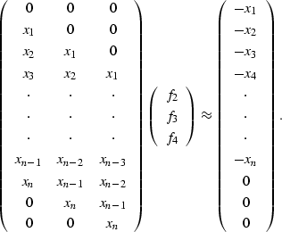
Notice how the matrix $\st A$ is made up of the vector $\sv x$ shifted against the filter to produce the convolution of $\sv x$ and $\sv f$.At least one element of $\sv f$ is constrained to be non-zero to prevent the trivial solution where all elements of $\sv f$ are zero. In this case, f₁ is constrained to be one so we can modify the equation above to move the constrained portion to the right-hand side to get

$$\left( \begin{array} {cccc} 0 & 0 & 0 \\ x_1 &0 & 0 \\ x_... ...\ \cdot \\ \cdot \\ -x_{n} \\ 0 \\ 0 \\ 0 \end{array} \right).$$ (42)

The new matrix without the first row will be referred to as $\st B$, and the set of filter coefficients without f₁ will be referred to as $\sv f'$.The system to be solved is then $\st B \sv f' \approx -\sv x$.Using the normal equations, the solution for $\sv f'$ becomes $\sv f' = (\st B^{\dagger} \st B)^{-1} \st B^{\dagger} (-\sv x)$.

$\st B^{\dagger} \st B$ is the autocorrelation matrix, which is also referred to as the inverse covariance matrix. The reason for calling $\st B^{\dagger} \st B$ an autocorrelation matrix is obvious, since the rows of the matrix are the shifted autocorrelation of $\sv x$.The description of $(\st B^{\dagger} \st B)^{-1}$ as a covariance matrix comes from the idea that $\sv x$ is a function of random variables. The relationship between the values of $\sv x$ at various lags are described by the expectation E of the dependence of the values of $\sv x$ with different delays. This is expressed as E(x_i x_j), where i and j are indices into the series $\sv x$.If the expectation E(x_i x_j) is zero when $i \neq j$,the spectrum of $\sv x$ would be white, and the sample values of $\sv x$ would be unrelated to each other. The autocorrelation would be zero except at zero lag.

The solution for $\sv f$ requires storing only the autocorrelation of $\sv x$and can be solved quickly and efficiently using Levinson recursion. Once again, the efficiency of this technique depends on $\st B^{\dagger} \st B$ being Toeplitz, which in turn depends on the type of convolution being transient, rather than internal or truncated-transient. When $\st B^{\dagger} \st B$ is not Toeplitz, it can still be solved using techniques such as Cholesky factorization, but at a higher cost of storage and calculation.