


The rapid processing of a huge amount of data requires us to simplify complex algorithms. Under the constant velocity assumption, the formulation of the dip moveout correction reduces to the equation for an ellipse. Because its expression remains simple in three dimensions, the process is computationally efficient. However, in the case of an irregular data acquisition geometry, the chaotic spatial spreading forbids a trace-parallel implementation.
After discussing the amplitude and phase of the elliptic dip moveout operator, I propose an efficient time-parallel implementation that allows a fast processing for any azimuthal distribution in the data.
Amplitude analysis of the constant-velocity anti-aliasing
three-dimensional integral dip moveout operator
A method of three-dimensional integral dip moveout processing for constant-velocity media must cope with problems related to amplitude and aliasing. The convolution of the dip moveout operator with triangle functions avoids the aliasing effect. A study of different amplitude weightings leads to the choice of the weighting scheme derived from a Fourier domain expression of dip moveout (). Testing the method on a 3-D synthetic data set shows the conservation of the amplitude-versus-offset (AVO) effect throughout the dip moveout (DMO) process.
Introduction
The Fourier domain DMO methods give appropriate results for 2-D lines but are time-consuming. In 3-D surveys, their implementation becomes more difficult because the spatial sampling rate as a function of azimuth is variable and irregular. In contrast to Fourier domain DMO methods, the integral DMO method is not affected by this problem and provides cheap processing because of the limited extent of the operator (which is two-dimensional and dip-limited). However, the implementation of an integral method requires explicit knowledge of the operator as well as of the weight applied to each operation. The next section describes the shape of the operator, and the second section states three rules that the DMO operator must satisfy.
The shape of the operator
Deregowski thoroughly described the elliptic DMO operator; I include Figure (Shape) only for the sake of introducing the terminology used throughout this paper.
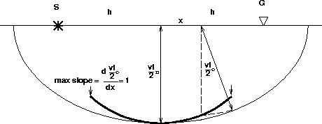 |

The operator is a dip-limited ellipse defined by the equation
| |
(1) |
The rules the operator must obey
The primary attribute of an integral method is to respect the kinematic component of the process. However, in order to yield a consistent stack of the operators illuminating a given location, the integration should be a weighted sum. In other words, an amplitude function should be applied along the operator. The integral DMO process will be consistent if it obeys the following rules.
Rule 1. According to Hale , ``The impulse responses [obtained by Fourier Transform DMO] may be used as a standard by which to judge integral DMO methods''. Because (f,k) DMO methods have a perfect behavior with respect to amplitude, the integral DMO operator should be as close as possible to the (f,k) DMO operator in amplitude and phase. Thus, we expect the integral impulse response to have a low amplitude and a high-frequency content near x=0 and a high amplitude and a low-frequency content when the slope of the operator becomes steeper.
Rule 2. Flat events must not be affected in amplitude and phase by the DMO process. This rule, clearly stated by Hale , is perfectly respected by any (f,k) DMO process (, ), but it represents a challenging test for integral DMO processes.
Rule 3. Events of a given reflectivity must show balanced amplitude after the DMO process, whatever their dip. This rule is essential in order not to spoil the data for a possible AVO study.
The first section of this part explains how to avoid the aliasing of the operator. In the next section, the three rules stated above help us choose the most convenient weighting among three amplitude schemes selected from the literature. Finally, a brief section discusses how to apply the operator on a 3-D grid.
The triangle as an anti-aliasing structure In the Fourier domain, the operator is not aliased. However, space-time integral methods must be applied carefully to account for operator aliasing.
For a given temporal frequency of the data, the increase in the dip of the operator produces an increase in the spatial frequency until it reaches the Nyquist frequency (two points per wavelength). Beyond that point, the operator is aliased.
Claerbout introduced an
efficient technique to avoid the aliasing of the operator
with Kirchhoff methods. Instead of spreading a simple spike along
the operator, a dip-dependent triangle is effectively convolved with
the operator. Assuming spatial spacing of ![]() , the width of
the triangle at a point of the operator is determined by
equation (2)
, the width of
the triangle at a point of the operator is determined by
equation (2)
| |
(2) |
Figure (Iraa) shows the impulse response of a spike when the triangle anti-aliasing method is used. The phase shift caused by the half differential filter (usual in 2-D Kirchhoff methods) makes the triangles look like the teeth in a shark's jaw.
|
Iraa
Figure 2 Impulse response of the anti-aliasing integral DMO using triangles. Input spike: 1.0 s; velocity: 2000 ms-1. | 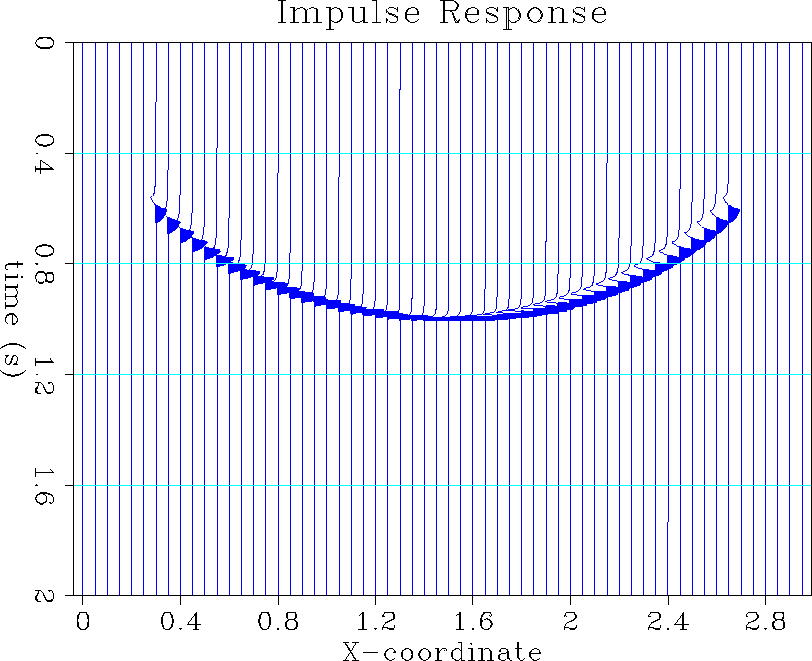 |
The triangular weight can be built with three spikes
![]() separated by
separated by ![]() and
submitted to both causal and anticausal integration. As
Figure (triangle) shows, the anti-aliasing process is cheap
because each output trace is double integrated only once.
and
submitted to both causal and anticausal integration. As
Figure (triangle) shows, the anti-aliasing process is cheap
because each output trace is double integrated only once.
|
triangle
Figure 3 Decomposition of the method for building triangles. All lines are equivalent: a triangle function is the convolution of two box functions (line 1 to 2); a box function is the integration of a two-opposite-spike signal (line 2 to 3); the convolution is commutative (line 3 to 4); the convolution of two two-opposite-spike signals is the final three-spike signal (line 4 to 5). The width | 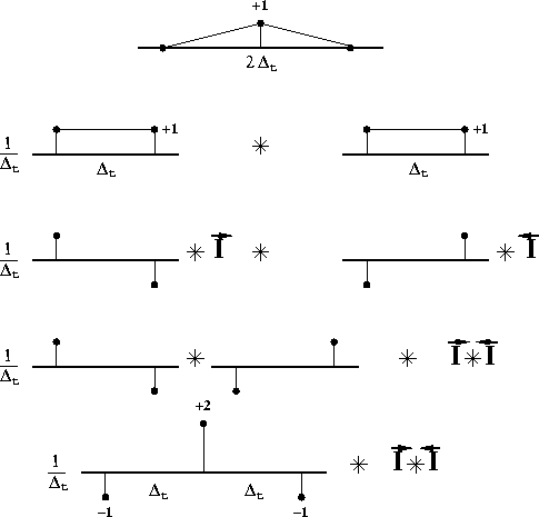 |
Amplitudes along the DMO operator A rich literature has been published describing ``true'' DMO amplitudes, which suggests that the truth is variable! In this section, I examine three propositions for amplitude weighting (, , ) to find the one that best verifies the rules stated in the introduction. I then discuss the inclusion of factors accounting for the spherical divergence and the effect of anti-aliasing on amplitudes.
Different weighting schemes
The weighting scheme proposed by Beasley
is based on a heuristic approach. Starting from the dip-domain
formulation of DMO (), he showed that the
amplitudes along the DMO operator are proportional to its curvature
![]() . Then he constrained the amplitudes in
time and offset to verify Rule 2, assuming a dominant frequency
of the data. He came up with the following expression:
. Then he constrained the amplitudes in
time and offset to verify Rule 2, assuming a dominant frequency
of the data. He came up with the following expression:
 |
(3) |
Gardner introduced the DMO-NMO method and derived a DMO amplitude factor that is directly related to the curvature of the operator through the expression
 |
(4) |
 |
(5) |
|
Amp
Figure 4 Normalized weighting schemes compared to (f,k) DMO amplitudes. Dotted line: Beasley; Dashed line: Gardner; Dashed-dotted line: Black; Solid line: picked amplitudes on the (f,k) DMO operator. | 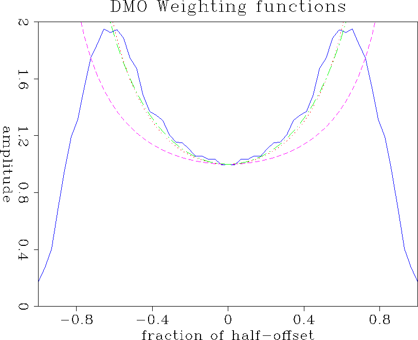 |
I now apply the rules to the three weighting schemes and compare their results.
Rule 1. Figure (Amp) shows the comparison of the different weighting schemes normalized by their value at x=0 with the amplitude picked along the impulse response of an (f,k) DMO program (Zhang's formulation). The different curves agree in shape, their concavity turned upward. However, Black's and Beasley's schemes are closer to the (f,k) DMO amplitudes. The decrease in amplitude of the (f,k) amplitude when x increases is caused by the velocity-dependent dip limitation of the operator. The three weighting functions have been plotted up to x=h without taking the limitation into account.
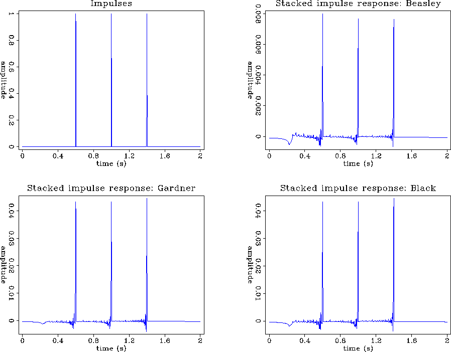
Rule 2. Figure (Imp) shows impulse responses that have been stacked along the x-axis. This stack simulates the contribution of impulse responses along a horizontal planar reflector to a single trace. Thus, to obey the second rule, the stacked impulse response should yield the input impulse. The three weighting schemes restore the balanced amplitudes of the impulse rather well. However, Gardner's and Black's schemes show a better stack, especially at earlier times, where Beasley's weighting produces strongest artifacts.
 |
Rule 3. In order to verify the third rule, I used a 3-D synthetic dataset created by David Lumley. Figure (Nmo) shows an NMO-corrected section of the model for a shot located at x = 0. The structure is composed of three planar reflectors: a horizontal reflector showing some amplitude effect (the amplitudes increase away from the source) and two shallow, dipping reflectors (15 and 30 degrees).
|
Nmo
Figure 6 A slice in the 3-D data after NMO. The horizontal plane shows some amplitude effect. The two other planes dip at a 15-degree and a 30-degree angle, respectively. | 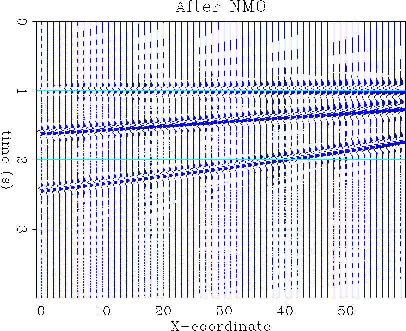 |
Figure (Dmo1) shows the result on the same section after the 3-D DMO. Some strong artifacts appear above the horizontal reflector, and the amplitudes are not well balanced along the reflectors or in relation to each other. This poor result is mainly caused by omission of spherical spreading and the amplitude-boosting effect of the anti-aliasing triangles.
|
Dmo1
Figure 7 A slice in the 3-D data after DMO with Black's amplitudes, without spherical spreading and without triangle effect corrections. | 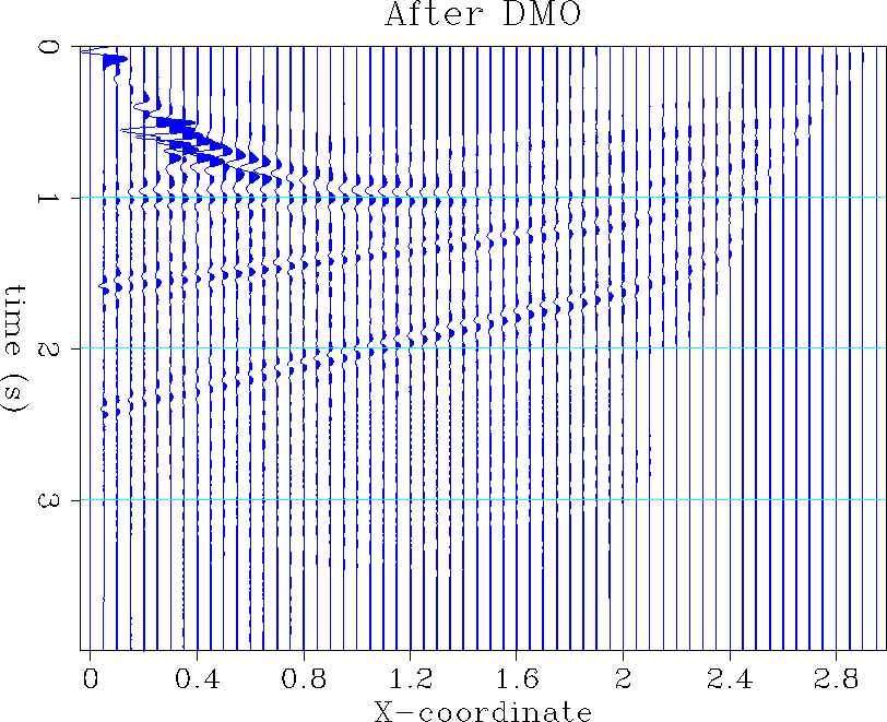 |
Spherical divergence
As suggested by the preceding result, spherical divergence should be included in the DMO process. Indeed, for a given shot-geophone traveltime, the zero-offset ray path when the reflector is dipping is shorter than when the reflector is horizontal. Since the decrease in amplitude of a spherical wave is inversely proportional to the distance traveled, the spherical spreading is clearly related to the dip of the structures and, thus, must be included in the DMO process.
Gardner expressed the spherical
spreading factor as a function of k (![]() ) and
t2 (t0). As a function of h, tn, and x, it becomes
) and
t2 (t0). As a function of h, tn, and x, it becomes
| |
(6) |
The effect of the anti-aliasing triangle width
The anti-aliasing is performed by effectively convolving a triangle function
with the output trace. The width of the triangle, ![]() , usually
exceeds the time sampling rate,
, usually
exceeds the time sampling rate, ![]() , for the steepest dips.
Therefore, the triangles overlap and produce an undesirable
amplitude increase. The number of overlapping triangles is
proportional to their width. Thus, a reasonable method of amplitude
correction is to divide the convolution triangles by
, for the steepest dips.
Therefore, the triangles overlap and produce an undesirable
amplitude increase. The number of overlapping triangles is
proportional to their width. Thus, a reasonable method of amplitude
correction is to divide the convolution triangles by ![]() , as
follows:
, as
follows:
| |
(7) |
|
Dmo2
Figure 8 A slice in the 3-D data after DMO with Black's amplitudes, corrected for spherical spreading and the triangle effect. |  |
Figure (Dmo2) shows the same section of the 3-D cube as Figure (Dmo1), but the DMO process now involves the two correction factors for spherical spreading and triangle width. The amplitude effect along the horizontal reflector is restored, and the relative amplitude of the different reflectors is better balanced and closer to the amplitude distribution in Figure (Nmo). The third rule is now more completely verified although some singularities occur at the near offset traces (close to x = 0).
The DMO operator in three dimensions As described by Hale , the zero offset rays bouncing off an ellipsoidal reflector of foci S (source) and G (geophone) emerge on the segment [SG]. Therefore, the DMO operator is really a 2-D operator working along the source-geophone line, even in a 3-D space. Consequently, applying the operator in three dimensions is not much different than in two dimensions except that the trace smearing is performed for an irregular spatial sampling according to the azimuth. The technique used in this 3-D DMO code consists of computing the bins affected by the segment [SG]. More precisely, whenever the center of a bin is closer to the [SG] segment than half the bin size, the bin receives an output trace. This operation is repeated for all input traces, gradually filling the output space. This technique is equivalent to the nearest neighbor interpolation in space and linear interpolation in time described by Nichols . This algorithm requires some evenly distributed data so that the fold over any bin is nearly constant. Dividing the trace amplitude by the fold of the corresponding bin seems an attractive solution, but it may spoil the amplitude properties of the data.
Conclusion
I implement a three-dimensional integral dip moveout processing algorithm for constant-velocity media that prevents operator aliasing. The study of amplitudes led me to choose Black's formulation as the most satisfactory in regard to three rules that assure the proper behavior of the DMO process. The method also corrects for spherical spreading.
Although the program has not been tested on real 3-D data, the results with synthetic data, especially regarding amplitude restoration, are encouraging. The next step consists of implementing the algorithm on the Connection Machine.
A parallel implementation of Kirchhoff DMO
In this section I compare two parallel algorithms for three-dimensional Kirchhoff dip moveout in a constant velocity medium. In the case of 3-D land data, an algorithm where data are processed in time slices allows highly irregular offset geometry. This mapping of the data into processor memory minimizes the cost of communication, which is reduced to nearest neighbor communication of time slices, and achieves load balance, keeping 80 percent of the processors busy throughout the process. The time aliasing of the operator is solved by a spatial convolution with dip-dependent triangles in two dimensions and with dip-dependent pyramids in three dimensions.
Introduction
Over the last years, DMO has become a standard step in seismic processing flows. The main reason for this is that it clearly improves the stack for little extra computational cost. Recently, some research showed that the improvement is even more distinct when depth-variable velocity is considered in the DMO process (, , ). However, these new methods are computationally expensive and a constant-velocity DMO is often enough to give an idea of the geological structures involved or improve the velocity analysis. Therefore, a parallel implementation of constant-velocity DMO is natural to reduce the processing time cost.
In a 3-D constant-velocity medium, the DMO process uses a line operator (). It convolves the input data with elliptical impulse responses, and sums the convolved data into the final stacked volume. The single dimension of the operator as well as its dip limitation are two reasons to consider 3-D constant-velocity DMO as a fast process whatever the geometry of the data acquisition. Unfortunately, the multi-azimuthal distribution of 3-D land data is a major obstacle for parallel implementation ().
This section details two possible parallel algorithms for 3-D constant-velocity DMO. The first algorithm involves a spiral data movement that does not use the full computational capabilities of the Connection Machine (CM5). The second algorithm reduces the communication cost by processing time slices but requires additional care to avoid temporal aliasing of the operator.
First algorithm: DMO by spiral data movement
The parallel implementation of DMO in a two-dimensional space is straightforward. Biondi describes a simple algorithm where the traces are laid out local to each processor. The DMO process then consists of a trace stretch and a nearest neighbor shift along the midpoint axis.
In three dimensions, the data shift is not restricted to a single axis but requires a movement of the input traces across a two-dimensional space. Biondi uses the same layout to apply DMO to 3-D marine data. The algorithm takes advantage of the regular data movement in the in-line direction because of the uniform sampling of the shot locations. However, 3-D land surveys record shot profiles of varying geometry (an example is shown in Figure (land3d)), and thus, the shot axis can not be processed in parallel.
|
land3d
Figure 9 This simple 3-D land acquisition geometry exhibits the non-recurrence of the shot profiles. As opposed to marine surveys, the geophone line does not move along with the shot location. |  |
Memory layout
Since the irregularity of 3-D land data appears in both azimuth and offset distributions, there is no preferential direction for data movement. Hence, Biondi had the idea of a spiral data movement alternating the shifts along the x- and y- axes. The algorithm can be outlined as follows:
|
spiral
Figure 10 Spiral pattern for data movement over output space. The shaded squares represent the processors that actually perform the stretch and the stack to the output. The white squares represent the processors that stay idle during the movement of the trace. | 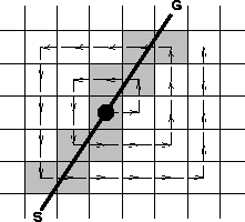 |
Load balance
By sorting the data into classes of offset, we can restrict the size of the spiral to the maximum offset of each class. The spiral data movement allows any azimuth distribution of the input traces. However, because a trace contributes to the stack only along its original source-geophone line, some processors are left idle during the spiral trip of the trace. Figure (spiral) shows the working processors in grey and the idle processors in white. In this example, the computer load, defined as the ratio of the number of working processors to the total number of processors, is thirty percent. For larger offsets, the load balance is expected to be worse because the number of working processors increases in proportion to the offset length whereas the total number of processors increases in proportion to the square of the offset. The unoptimized use of processing power makes the algorithm inefficient for 3-D land data.
Second algorithm: DMO by time slice
In order to spread the data along an elliptical path in (t,x,y) space, it is possible to either move spatially from bin to bin and stretch the traces or move the time slices upward and stretch the data in the offset direction.
Memory layout
The memory layout for processing time slices is illustrated in Figure (tsproc). The time slices are local to each processor and the time axis is the parallel dimension. Thus, the number of processors needed is the number of time samples, and the memory of each processor must be large enough to load and process one time slice. When the amount of data exceeds the memory available, the process can run on blocks of data. The blocks may be pieces of data cut in the (x,y) space, preserving the parallel axis and relieving the processors memory, or they may be cut in time, shortening the parallel axis but requiring a smaller area of overlap between successive lumps.
|
tsproc
Figure 11 The top-most drawing represents the elliptic dip-limited DMO operator. I assume that the offset line bisects the x- and y- axes on the Earth's surface. Below, the two grids represent the data layout inside the processors. Each processor contains a time slice of data. Processor 1 contains the time slice at t=t0 and performs the data communication across the (x,y) space that corresponds to a vertical shift from t0 to t1. During this time, processor 2 performs the same kind of operation for a vertical shift from t1 to t2. Then, processor 1 sums its output in the output volume and communicates its input to processor 2. The action is then repeated, moving the data across the (x,y) space for a vertical shift from t0 to t2. | 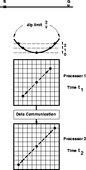 |
Unlike the previous algorithm, data communication is performed in a single direction, up the time axis, and does not depend on the offset and azimuth distribution. The long ranging and chaotic communications in the (x,y) space take place in-processor. Thus, the processing of time slices results in a more efficient inter-processor communication than the trace processing.
Load balance
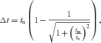
Because the DMO elliptic operator is dip-limited, it does not extend all the way up to the Earth's surface (t=0). The time spread of the impulse response is given by:
 |
(8) |
|
magic
Figure 12 Time spread of the impulse responses of DMO as a function of the impulse location, tn. The maximum time spread occurs for the input time | 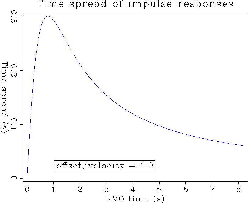 |
An interesting feature of these curves is that the time spread
of the impulse responses never exceeds ![]() where
where ![]() is
is
| |
(9) |
During the process, the time slices are shifted upward until they reach the maximum time spread. Of course, only the time slice corresponding to the maximum time spread will have to be processed all the way. Other time slices, like for example tn=5 seconds (Figure (magic)), will be processed for the first .1 second and then pass through idle processors. Obviously, the later time slices require less processing than the earlier ones, and thus represent a waste of processing capacity. The following formula gives the load balance as a function of trace length:
| |
(10) |
|
integ
Figure 13 Load balance as a function of the trace length. The optimal load balance of eighty percent corresponds to a trace length which is a function of tm (=2h/v). The bigger tm is, the later the load balance is optimal. Click on the following button to see a movie of the load balance for different values of tm. | 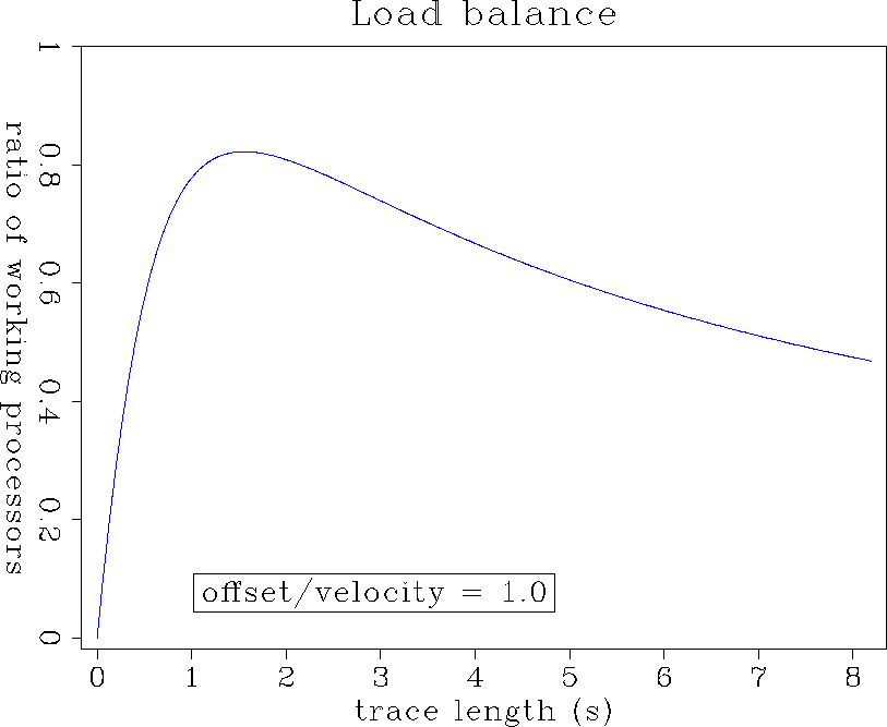 |
This algorithm allows a more efficient distribution of work between processors than the spiral trace processing described earlier. I implemented this algorithm for a two-dimensional model (Figure (res) is an output of the program) but the run time is similar to a serial implementation of DMO (in 2-D, trace processing is more straightforward than time-slice spreading). However, the real advantage of the method will appear in processing 3-D land data.
The pyramid as an anti-aliasing structure
Applying DMO in time slices assures that the operator will not introduce spatial aliasing in the data. However, the spatial spreading from one time slice to the next must never exceed the bin spacing or temporal aliasing will occur, especially for the gentle dips of the operator ().
A technique described by Claerbout prevents operator aliasing. The method consists of the convolution of the operator with triangles whose width depends on the dip of the operator as described previously. However, this process differs from the trace-oriented process in that the convolution is applied horizontally in the time slices. Figure (res) shows the DMO response of several impulses corrected with anti-aliasing triangles.
|
res
Figure 14 Impulse responses of DMO applied to time slices. The anti aliasing triangles are wide at gentle dips and shrink towards the steepest dips. |  |
In three dimensions, the triangles cannot be directly obtained by Claerbout's double integration technique. Instead, a similar method leads to the construction of pyramids in a three-dimensional extension of the concept of the triangle. Figure (pyramid) shows how to decompose the construction of a pyramid. The pyramids cause a lateral expansion of the operator that does not agree with the theoretical ellipse of dip moveout. However, the operator has a cross-line component when we consider variable velocity or transversely isotropic media. Gonzalez showed that the three-dimensional DMO operator in the cross-line direction may curve either downward when the velocity increases with depth or upward when the velocity increases with angle in a transversely isotropic medium. In both cases, the first derivative of the operator with respect to the cross-line coordinate vanishes on the in-line axis. Therefore, the horizontal expansion caused by the pyramids is a first-order approximation of the operator.
|
pyramid
Figure 15 Decomposition of the method for building pyramids. All lines are equivalent: a pyramid function is the convolution of two box functions (line 1 to 2); a box function is the x-integration of an x-opposite-spike square signal (line 2 to 3); an x-opposite-spike square signal is the y-integration of an x-y-opposite-spike square signal (line 3 to 4); the convolution is commutative (line 4 to 5); the convolution of two x-y-opposite-spike square signals is the final nine-spike signal (line 5 to 6). The dimensions | 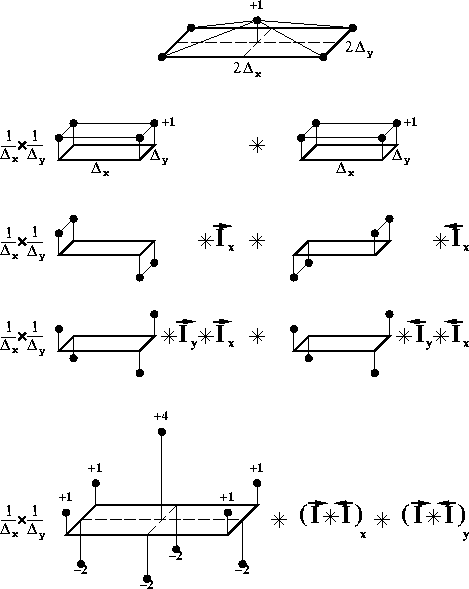 |
Because constant-velocity DMO in a 3-D Earth model operates along curves, care must be taken in parallel implementation in order to avoid the waste of computational capacity. Trace processing algorithms require a great deal of inter-processor communications and leave many processors idle during the process. On the other hand, the processing of time slices is well adapted to the irregular geometry of 3-D land data, attaining a load balance of eighty percent. Although the anti-aliasing convolution is more quickly performed along traces, the efficient use of computational capacity compensates for a slower convolution in the time slices. Unfortunately, the three-dimensional implementation of the time-slice algorithm has not been tested on real data. Doing so would tell us whether the lateral expansion of the operator is an undesirable artifact or a step toward the variable-velocity assumption.