previous up next print clean
Next: Computer time requirements Up: TWO-DIMENSIONAL LATERAL PREDICTION Previous: Comparison of two-dimensional f-x

The biasing of f-x prediction toward the output point

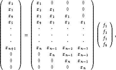
Though less of a problem than the long time-length filter, the tendency for the lateral prediction coefficients to be concentrated near the output trace position with Gulunay's f-x prediction causes more noise to be passed. The source of this problem can be seen in the system describing the f-x prediction filtering, $ \sv d= \st X \sv f$, or  
 \begin{displaymath}
\left(
\begin{array}
{c}
 x_2 \\  x_3 \\  x_4 \\  x_5 \\  \c...
 ...in{array}
{c}
 f_1 \\  f_2 \\  f_3 \\  f_4 \end{array} \right),\end{displaymath} (6)
where the vector $\sv d$ is the desired output, $\st X$ is the input data shifted with respect to the filter, and $\sv f$ is the filter to be calculated. The zeros in the last few coefficients of $\sv d$ tend to reduce the f2,f3, and f4 coefficients of the filter. The zeros at the top of the $\st X$ matrix have a similar effect. The result of this tendency to weight the f-x prediction filter coefficients toward the output point of the filter may be appealing in terms of producing an output trace made up of the nearest traces, but the noise in the nearest traces is also passed with less attenuation. This increased weighting of the nearest traces produces a filter that is less effective in rejecting noise.

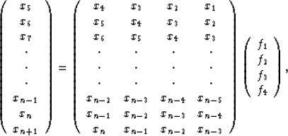
The increased weighting of the nearest trace can be remedied by setting up the problem differently. Removing the top and bottom rows of Equation (6) produces  
 \begin{displaymath}
\left(
\begin{array}
{c}
 x_5 \\  x_6 \\  x_7 \\  \cdot \\  ...
 ...gin{array}
{c}
 f_1 \\  f_2 \\  f_3 \\  f_4\end{array} \right),\end{displaymath} (7)
so the filter is calculated only where nonzero data are available. Unfortunately, the normal equations $\sv f = (\st X^{\dagger} \st X)^{-1} \st X^{\dagger} \sv d$cannot be used, since $(\st X^{\dagger} \st X)$ does not necessarily have an inverse. For a flat event, all the coefficients in the $\st X$ matrix have equal values, and all the elements of $\st X^{\dagger} \st X$also have equal values, making $\st X^{\dagger} \st X$ singular.

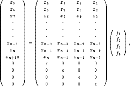
Expanding Equation (7) to add a damping condition to equally weight the filter coefficients gives  
 \begin{displaymath}
\left(
\begin{array}
{c}
 x_5 \\  x_6 \\  x_7 \\  \cdot \\  ...
 ...gin{array}
{c}
 f_1 \\  f_2 \\  f_3 \\  f_4\end{array} \right),\end{displaymath} (8)
where $\epsilon$ is a small number. Solving this set of equations avoids the tendency for the largest coefficients to cluster near the output position that we have seen in Gulunay's method.

Although these modifications should improve the noise attenuation properties of the complex prediction filter, the biasing effect on the noise attenuation is very small compared to the improvement from using the shorter time-length filter of a typical t-x prediction. A feature of Gulunay's method is, that for noiseless data, prediction is unneeded and concentrating the strongest predictions coefficients near the output has no effect on the results. As the strength of the noise increases, the distribution of the amplitudes of the filter coefficients becomes more even, since adding noise to the input provides the same effect as adding a factor to the diagonal of $\st X^{\dagger} \st X$.

It might be thought that this noise-dependent coefficient weighting gives f-x prediction an advantage over t-x prediction. However, if an irregularity such as a fault exists in the input data, both t-x and f-x predictions will generate identical filters in the noiseless case, since the difference between the input and the predicted data will be smallest for a filter with strong filter coefficients adjacent to the output trace and producing the least smearing of the irregularity. For perfectly regular data with noise added, the f-x prediction filter coefficient distribution will approach that of the t-x prediction filter as the strength of the noise is increased. Thus f-x prediction always has an effectiveness that is less than or equal to the t-x predictions effectiveness.


previous up next print clean
Next: Computer time requirements Up: TWO-DIMENSIONAL LATERAL PREDICTION Previous: Comparison of two-dimensional f-x
Stanford Exploration Project
11/16/1997