The relationship of f-x prediction to t-x prediction

When applied to data with relatively mild random noise problems, most of the cases where t-x prediction was compared to f-x prediction showed practically identical results. In tests on synthetics with simple flat or dipping events in the absence of noise, both techniques passed events without distortion. These same simple cases with an added background of relatively low-amplitude random noise also produced comparable results. The results using real data sets with both techniques were also similar. Differences appeared only when the energy of the noise became a significant fraction of the energy of the signal.

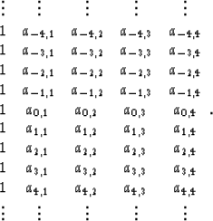
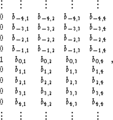
These similarities and differences are explained by comparing the form of the t-x prediction filter and the form of the effective t-x domain filter created by f-x prediction. The individual filters calculated by the f-x prediction have the form  

$$\begin{array} {ccccc} 1 & a_{1} & a_{2} & a_{3} & a_{4} \end{array},$$ (3)

where a₁,a₂,a₃, and a₄ are complex numbers. Collecting these filters and presenting them in the frequency-space domain produces the following composite filter:

$$\begin{array} {ccccc} \vdots & \vdots & \vdots & \vdots & \... ...,4} \\ \vdots & \vdots & \vdots & \vdots & \vdots \end{array}.$$ (4)

Transforming this filter from the frequency-space domain into the time-space domain gives the effective t-x domain filter

$$\begin{array} {ccccc} \vdots & \vdots & \vdots & \vdots & \... ...,4} \\ \vdots & \vdots & \vdots & \vdots & \vdots \end{array},$$ (5)

where the number of rows is the number of time samples in the window being considered. The Fourier transform has converted the first column of 1s into a single 1 at the output position, creating a time-space filter with the same form as the t-x prediction filter shown in (1), but with the number of rows greatly increased.

For data with random noise that has low amplitude compared to the signal, the coefficients of the filter producing most of the prediction are expected to lie close to the center of the filter in time, since events far from the output point in time are unlikely to affect data at the output position. For data with high amplitude random noise, random correlations of events widely separated in time create undesirable lineups with significant amplitudes in the output of f-x prediction. Since the f-x prediction produces a very long effective t-x filter in time, its prediction is contaminated with random correlations, where the t-x prediction, with its smaller filter, is not.

The time-length problem of the f-x prediction filter can be compared to the problem of calculating a one-dimensional prediction filter from a short time series. If a long one-dimensional prediction filter is calculated and applied to a short time series, practically everything in the time series will be predicted. Having a two-dimensional filter with a significant lateral width compensates for some of this overprediction, but a short t-x prediction filter is a more complete solution to the problem.

Another effect of the long time-length filter in f-x prediction is the generation of false events. If two strong parallel events are embedded in a background of random noise, f-x prediction generates weak, but significant events parallel to the strong events. While both t-x and f-x techniques tend to line up noise with strong events, f-x prediction actually generates false events with its long filter in time. These spurious events occur because parallel events in a random noise background produce an f-x filter where the prediction of one strong event is influenced by the presence of other parallel events. The t-x prediction is much less likely to be affected by the influence of widely separated events because of its short filter in time.