


An f-x prediction like FXDECON
predicts linear events in the
frequency-space domain. A linear event, given by the expression
![]() ,where x is the lateral position and t is
time, is Fourier transformed in time into
,where x is the lateral position and t is
time, is Fourier transformed in time into
![]() or
or ![]() . For a simple linear event,
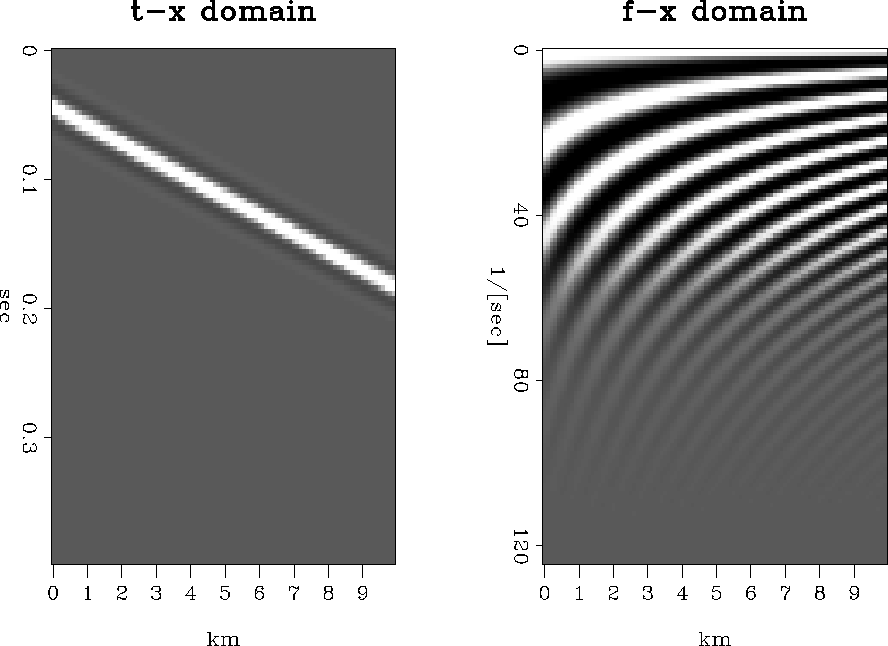
this function is periodic in x.
This periodicity can be seen along any constant frequency line
in the f-x domain display in Figure 1.
. For a simple linear event,
this function is periodic in x.
This periodicity can be seen along any constant frequency line
in the f-x domain display in Figure 1.
 |


To predict a linear event in ![]() ,where
,where ![]() is a sampled version of
is a sampled version of ![]() for a single frequency,
Gulunay1986 proposed calculating a least-squares
prediction filter
for a single frequency,
Gulunay1986 proposed calculating a least-squares
prediction filter ![]() from the system
from the system
![]() , or, as expanded,
, or, as expanded,
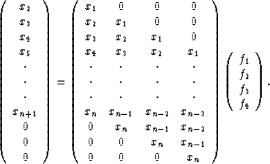 |
(2) |
The input to the prediction problem is the data
from a
single frequency over the width of the window in space.
This input
is a set of complex numbers
![]() .The desired output
.The desired output ![]() is
is
![]() ,a one-sample step-ahead prediction of the input.
While
,a one-sample step-ahead prediction of the input.
While ![]() can be built with a longer shift of the input data, a
shift of one sample is generally used.
Notice that the desired output
can be built with a longer shift of the input data, a
shift of one sample is generally used.
Notice that the desired output ![]() starts with x2 and ends with
xn+1. Gulunay 1986
set up the problem using this extra element from
the input to guarantee that the filter would produce a result with the
same amplitude as the input regardless of the length of the filter
and of the data.
The rows of the matrix
starts with x2 and ends with
xn+1. Gulunay 1986
set up the problem using this extra element from
the input to guarantee that the filter would produce a result with the
same amplitude as the input regardless of the length of the filter
and of the data.
The rows of the matrix ![]() are shifted versions of the input
that produce a convolution
with the desired filter
are shifted versions of the input
that produce a convolution
with the desired filter ![]() .This filter
.This filter ![]() can be calculated using the normal equations
can be calculated using the normal equations
![]() ,where
,where ![]() indicates the
conjugate transpose, or adjoint.
This is a standard solution to least-squares problems,
except that the sample values are complex numbers, so the adjoint operation
indicates the
conjugate transpose, or adjoint.
This is a standard solution to least-squares problems,
except that the sample values are complex numbers, so the adjoint operation
![]() cannot ignore taking the complex conjugate of the matrix elements
on which it operates.
cannot ignore taking the complex conjugate of the matrix elements
on which it operates.
The f-x prediction is applied to small windows to ensure that events are locally linear, just as in the t-x prediction case, and the data within each window are then Fourier transformed. For the spatial series created at each frequency by the Fourier transform, a prediction filter is calculated as described in the preceding paragraph. Each calculated filter is first applied forward and then reversed in space, with the results averaged to maintain a symmetrical application, as in the t-x prediction case. The inverse Fourier transform is then applied to the filter result in each window, and the windows are merged to form the output image.
The calculation of the filter for each frequency is independent of the calculations of the filters for other frequencies. While the filters calculated at each frequency are a least-squares solution, this multitude of least-squares solutions does not necessarily produce a collective filtering action that is a global least-squares result. In the next section, we discuss the effect of this partitioning and the resulting differences between the actions of t-x prediction and f-x prediction.