![[*]](http://sepwww.stanford.edu/latex2html/foot_motif.gif) from familiar normal moveout equations
from familiar normal moveout equations
 |
(1) | |
| (2) |
![[*]](http://sepwww.stanford.edu/latex2html/cross_ref_motif.gif) .
Because of the limited alphabet of programming languages,
I used the keystroke z to denote
.
Because of the limited alphabet of programming languages,
I used the keystroke z to denote
subroutine nmo0( adj, add, slow,    x, t0, dt, n,zz,  tt )
integer  it, iz, adj, add,                        n
real  xs, t , z,           slow(n), x, t0, dt, zz(n), tt(n)
call adjnull(    adj, add,                     zz,n,  tt,n)
do iz= 1, n {	z = t0 + dt*(iz-1)		# Travel-time depth
		xs= x * slow(iz)
		t = sqrt ( z * z + xs * xs)
		it= 1 + .5 + (t - t0) / dt	# Round to nearest neighbor.
		if( it <= n )
			if( adj == 0 )
				tt(it) = tt(it) + zz(iz)
			else
				zz(iz) = zz(iz) + tt(it)
	}
return; end
subroutine adjnull( adj, add, x, nx,  y, ny )
integer ix, iy,     adj, add,    nx,     ny
real  			      x( nx), y( ny )
if( add == 0 )
	if( adj == 0 )
		do iy= 1, ny
			y(iy) = 0.
	else
		do ix= 1, nx
			x(ix) = 0.
return; end
The adjoint operation begins from a model like the zero-offset trace
and sprays this trace to all offsets.
The moveout and stack operations ![]() are done by subroutine stack0()
with the adj=1 argument
and the modeling operation
are done by subroutine stack0()
with the adj=1 argument
and the modeling operation ![]() is done by
subroutine stack0() with the adj=0 argument.
is done by
subroutine stack0() with the adj=0 argument.
subroutine stack0( adj, add, slow,     t0,dt, x0,dx, nt,nx, stack, gather)
integer ix,        adj, add,                         nt,nx
real     x,                  slow(nt), t0,dt, x0,dx,   stack(nt), gather(nt,nx)
call adjnull(      adj, add,                           stack,nt,  gather,nt*nx)
do ix= 1, nx {
	x = x0 + dx * (ix-1)
	call nmo0( adj, 1, slow, x, t0,dt, nt, stack, gather(1,ix))
	}
return; end
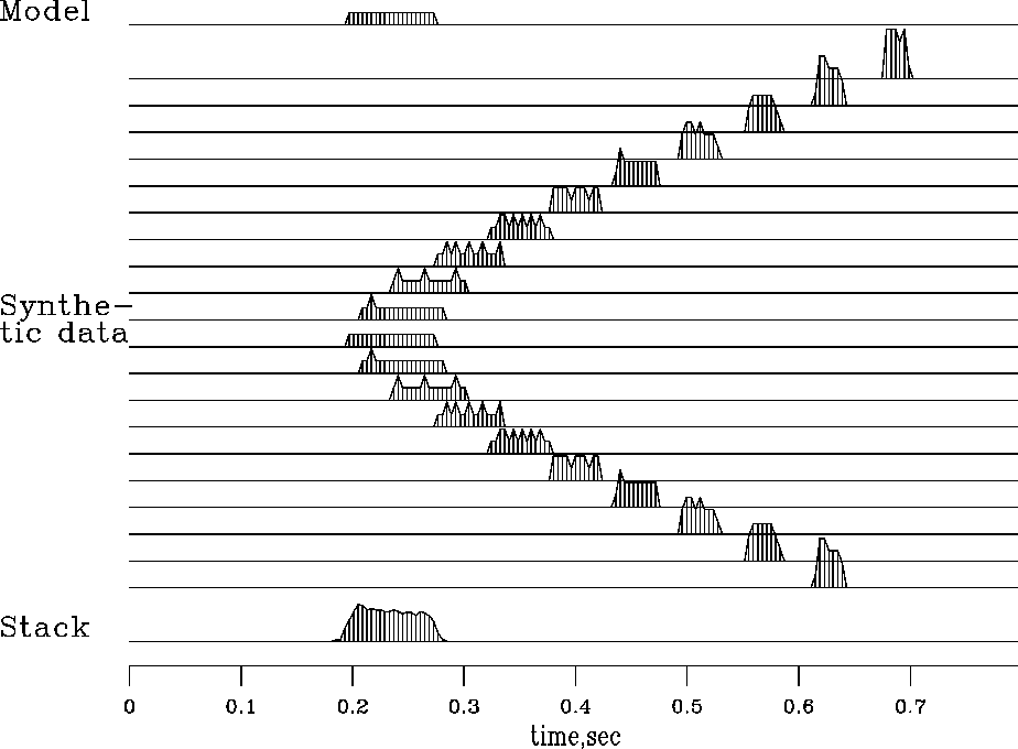
Figure 1 illustrates the modeling operator and its adjoint.
|
stack
Figure 1 Top is a model trace |  |
Notice the roughness on the waveforms caused by different numbers of points landing in one place. Notice also the increase of AVO (amplitude versus offset) as the waveform gets compressed into a smaller space. Finally, notice that the stack is a little rough, but the energy is all in the desired time window.
Parenthetically, we notice a contradiction of aspirations. On the one hand, an operator has smooth outputs if it ``loops over output space'' and finds its input where ever it may. On the other hand, it is nice to have modeling and processing be exact adjoints of each other. Unfortunately, we cannot have both. If you loop over the output space of an operator, then the adjoint operator has a loop over input space and a consequent roughness of its output.