


Next: ANELLIPTIC ANISOTROPY
Up: Ecker & Muir: Stolt
Previous: INTRODUCTION
The normal Stolt migration algorithm for the dispersion relation of the
scalar wave equation
|  |
(1) |
is implemented using the following equation to map from the ``data'' to the
``image'' space:
| 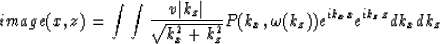 |
(2) |
where P(kx,w(kz)) is the fourier transformation of the data recorded at the
surface.
This equation can easily be transformed into the time domain by using the
relationship  between two-way traveltime
  , depth z
and vertical velocity vz and can be extended into:
, depth z
and vertical velocity vz and can be extended into:
|  |
(3) |
where
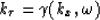
is a function of kx and  and
and  is the new Jacobian
depending now on
is the new Jacobian
depending now on  instead of kz.
Any desired dispersion relation can be put into this new generalized equation
by simply deriving the appropriate Jacobian and which can be
substitited in equation (3).
instead of kz.
Any desired dispersion relation can be put into this new generalized equation
by simply deriving the appropriate Jacobian and which can be
substitited in equation (3).
The Stolt migration algorithm for the extended imaging equation (3) can
then be represented as:

In order to determine the value  from
from  a mapping from the to the axis has to be performed.
In calculating , we require the value of which is calculated by a frequency-domain interpolation.
In this study, an exact interpolation scheme by Rosenbaum 1981
is implemented in the migration algorithm:
a mapping from the to the axis has to be performed.
In calculating , we require the value of which is calculated by a frequency-domain interpolation.
In this study, an exact interpolation scheme by Rosenbaum 1981
is implemented in the migration algorithm:
| ![\begin{displaymath}
C'(n+\delta n) = \sum_{m=0}^{N-1} C(m) e^{-\pi i[(n+\delta n) - m]} sinc[(n +
\delta n) - m]\end{displaymath}](img13.gif) |
(4) |
where N is the number of given points and the point to be interpolated lies at
the point  .In this interpolator the weights are the product of a sinc function and a
corkscrew function
.In this interpolator the weights are the product of a sinc function and a
corkscrew function ![$e^{-\pi i[(n+\delta n) - m]}$](img15.gif) .
Popovici et al. 1993
compare Rosenbaums technique with a slow Fourier transformation
in time for an irregular range of frequencies followed by an inverse Fourier
transformatio. This has been implemented on a parallel computer by Blondel
and Muir 1993.
.
Popovici et al. 1993
compare Rosenbaums technique with a slow Fourier transformation
in time for an irregular range of frequencies followed by an inverse Fourier
transformatio. This has been implemented on a parallel computer by Blondel
and Muir 1993.
Next: ANELLIPTIC ANISOTROPY
Up: Ecker & Muir: Stolt
Previous: INTRODUCTION
Stanford Exploration Project
11/16/1997