


Next: ADAPTION OF THE DERIVATIVE
Up: Karrenbach: Splitting the wave
Previous: Introduction
The constitutive equation
links basic wave propagation observables with the medium parameters.
Combining a force balance equation with a constitutive equation
results in a wave equation. In this exposition I use the elastodynamic
wave equation.
The constitutive equation and force balance without exterior forces
in a perfectly elastic medium are
|  |
(1) |
| (2) |
| (3) |
where u is the elastic displacement,  the strain,
 the stress and
  the stiffness tensor.
The resulting wave equation involves calculating tensor products and
derivatives. This wave equation operator L can be defined as
the stiffness tensor.
The resulting wave equation involves calculating tensor products and
derivatives. This wave equation operator L can be defined as
| 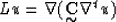 |
(4) |
 is a partial derivative operator matrix
acting on its argument. is the stiffness tensor
and u is the displacement field.
Using the chain rule for covariant derivatives and applying it
to the tensor product, we can rewrite equation (4) to
is a partial derivative operator matrix
acting on its argument. is the stiffness tensor
and u is the displacement field.
Using the chain rule for covariant derivatives and applying it
to the tensor product, we can rewrite equation (4) to
| 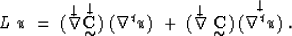 |
(5) |
The  pairs indicate the entity on which
the matrix of derivative operator is acting upon. In the first term of
equation (5) derivatives of the elastic constants are computed;
in the second term only derivatives of the strain tensor are computed.
The stiffness components in the second term act as constant coefficients
for the derivate matrix elements.
We can rewrite operator equation (5) in terms of its tensor elements
by using (1) and get
pairs indicate the entity on which
the matrix of derivative operator is acting upon. In the first term of
equation (5) derivatives of the elastic constants are computed;
in the second term only derivatives of the strain tensor are computed.
The stiffness components in the second term act as constant coefficients
for the derivate matrix elements.
We can rewrite operator equation (5) in terms of its tensor elements
by using (1) and get
| ![\begin{displaymath}
l_i = \sum_{jkl} [\ (\ {\partial_i\over{\partial_j}} +
{\p...
...+
\ {\partial_j\over{\partial_i}}\ ) \
{\bf\epsilon_{kl}}\ ]\end{displaymath}](img9.gif) |
(6) |
where [...] indicates the scope of the partial derivatives and
where  .Equation (6) is written in its most general form
and is valid for anisotropic media.
The derivative operation in equation (6)
appears in both terms. It acts, however, on two different entities.
In the first term the derivative of medium properties is taken
and in the second term the derivative of the wave field is computed.
In the end summation of both terms produces the complete derivative
without taking a derivative of the medium and wave field product,
as equation (4) would suggest.
For a medium with constant properties
the first term vanishes, leaving the second term in equation
(6), whose Fourier transform
represents the Christoffel equation.
From an economical point of view equation (6)
doesn't seem attractive, but the opportunity lies in
computing the solution to equation (4) more accurately and
more realistically for certain types of media.
In particular the properties of derivatives
can be adjusted to match the properties of the observables.
.Equation (6) is written in its most general form
and is valid for anisotropic media.
The derivative operation in equation (6)
appears in both terms. It acts, however, on two different entities.
In the first term the derivative of medium properties is taken
and in the second term the derivative of the wave field is computed.
In the end summation of both terms produces the complete derivative
without taking a derivative of the medium and wave field product,
as equation (4) would suggest.
For a medium with constant properties
the first term vanishes, leaving the second term in equation
(6), whose Fourier transform
represents the Christoffel equation.
From an economical point of view equation (6)
doesn't seem attractive, but the opportunity lies in
computing the solution to equation (4) more accurately and
more realistically for certain types of media.
In particular the properties of derivatives
can be adjusted to match the properties of the observables.
Next: ADAPTION OF THE DERIVATIVE
Up: Karrenbach: Splitting the wave
Previous: Introduction
Stanford Exploration Project
11/17/1997