REVIEW OF LITWEQ OPERATOR

LITWEQ method is based on the scalar wave equation for variable velocity media,  

$${\partial^2 P\over\partial x^2}+{\partial^2 P\over\partial z^2}= {1\over v^2(x, z)}~{\partial^2 P\over\partial t^2} .$$ (1)

The basic idea in this method is to rewrite the 2-D scalar wave equation in a new coordinate system. This allows us to produce uniformly space grids and to approximate the solution of (1) by using finite difference. First, let's define an auxiliary variable $\tau$ sometimes called pseudo-depth,

$$\tau=\int_0^z{1\over v(x,\theta)}d\theta.$$ (2)

Second, let's define a reference velocity to measure the lateral velocity variation in the media:

$${1\over v^2(z)}={1\over nx} \sum_{i=1}^{nx}{1\over v^2(x_{i},z)} ,$$ (3)

where nx represents the number of points in the common mid point direction. With the definitions above it is possible to rewrite (1) in terms of (2) and (3) as

$$\begin{eqnarray} {\partial^2 P\over\partial x^2}+{1\over v^2(\tau)} ({\partial^2... ...v^2(x,\tau)}-{1\over v^2(\tau)}) {\partial^2 P\over\partial t^2} ,\end{eqnarray}$$ (4)

where $v(\tau)$ and $v(x,\tau)$ are the corresponding v(z) and v(x,z) using the definition of $\tau$.

Equation (4) is defined on the $(X, \tau, t)$ domain which is independent of the velocity. This is because we have already integrated along it when defining $\tau$ in (2). Now, we are ready to define a linear transformation (independent of the velocity) that incorporates the solutions of (4) along their characteristic lines. The linear transformation is:

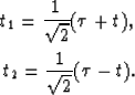$$\begin{eqnarray} t_1 = \frac{1}{\sqrt{2}} (\tau + t) , \\ t_2 = \frac{1}{\sqrt{2}} (\tau - t) .\end{eqnarray}$$ (1) (2)

Using the chain rule for scalar fields is easy to show the following relations for this particular transformation,

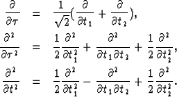$$\begin{eqnarray} {\partial\over\partial\tau} & = & {1\over\sqrt{2}}({\partial\ov... ...1}\partial t_{2}} + {1\over 2}{\partial^2\over\partial t_{2}^2} .\end{eqnarray}$$ (1) (2) (3)

Finally, using (5) and substituting (6) in (4) we get the LITWEQ operator:

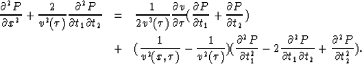$$\begin{eqnarray} {\partial^2 P\over\partial x^2} + {2\over v^2(\tau)} {\partial^... ...ial t_{1}\partial t_{2}} + {\partial^2 P\over\partial t_{2}^2}) .\end{eqnarray}$$ (7)

A detailed derivation of (7) is presented in Li (1986).