Imaging horizontal reflectors

On the above smooth background velocity model, I superimposed two horizontal reflectors. The reflector at a depth of 40 m is split at the horizontal position of 50 m vertically by 2 m, which is equal to half the dominant wavelength. The reflector at a depth of 160 m is split horizontally to generate a hole 22 m wide centered at the horizontal position of 50 m. The first Fresnel zone width at this depth relative to the source at a depth of 100 m on the left well is 22 m. I compute the Fresnel zone using Equation (8.2) (Yilmaz, 1987), which is valid for zero-offset surface surveys. The crosswell survey has a different geometry than a surface survey, and thus it should have a different formula to compute the Fresnel zone. However, I assume that the Fresnel zone width as computed by the formula valid for surface survey would not differ significantly from the true width of the crosswell Fresnel zone.

 

BackTimemap
Figure 2 A smooth background velocity model, in which high-wavenumber velocity heterogeneity reflectors will be superimposed. Overlayed on this figure is the direct wave traveltime contour map from the source.

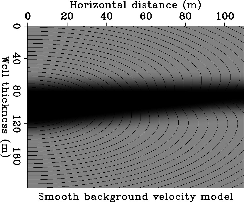
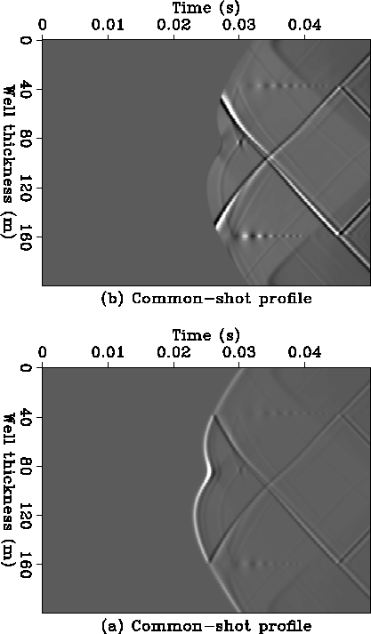
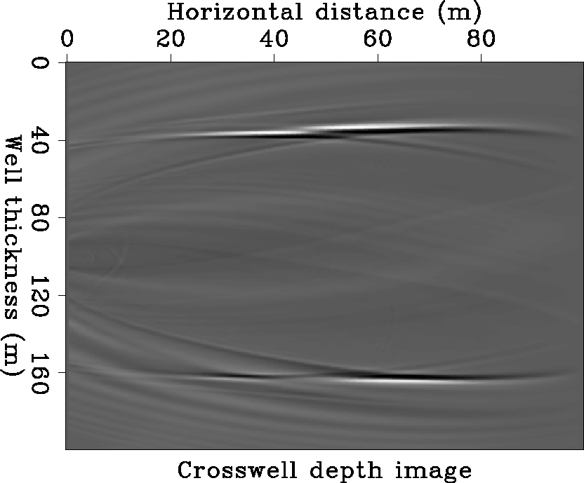
Figure 3(a) is the common-shot profile data generated by fourth-order-in-time, tenth-order-in-space finite-difference modeling with the source located at depth of 100 m in the left well and the receivers equally spaced at a depth interval of 0.5 m in the right well. Figure 3(b) shows the same common-shot profile data, but the direct wave has been muted because it does not help reflection imaging. The vertical faulting on the upper reflector and the horizontal faulting on the lower reflector have an effect of their reflection events. Figure 2 also shows the direct-wave traveltime contour map from the source computed by finite-difference method(Van Trier and Symes, 1990). It indicates the time that a diffractor is excited during modeling and also the time that the diffractor is imaged during migration wavefield backpropagation. With the recorded common-shot profile data as boundary conditions along the recording grid points, I run the two-way wave equation backward in time. Imaging is performed at each step of the wavefield extrapolation by extracting the values of the grid points that are imaged at that time as reflectivity and adding them into the image plane at the same locations. The locus of all points that are imaged at a particular time step corresponds to the direct wave exciting wavefront from the source. The common-shot profile data that are input for migration processing are without divergence corrections because of the reversibility of modeling-migration conjugacy, which is explained in Appendix A. Using fourth-order-in-time, tenth-order-in-space finite differencing to solve the wave equation for migration wavefield backpropagation, I should gradually drop the order of central spatial finite differencing to the second-order near the recording boundary for the derivative perpendicular to the recording boundary, in order to avoid edge oscillation and ensure that the numerical solution conforms to physical wave phenomena. The coefficients of the second to tenth order of central finite differencing for the second derivative are given in the Appendix B. Figure 4 shows the reflectivity depth image between the two wells. The half wavelength of 2 m vertical faulting at a horizontal position of 50 m on the upper reflector can be clearly interpreted. The existence of the 22 m wide horizontal hole on the lower reflector can only be inferred because its dimension is equal to the corresponding 22 m wide first Fresnel zone.

There are some small artifacts in the image background. These artifacts can be diminished by using the redundancy stack of muti-shot migration images. It is remarkable that only one shot migration can image the reflectivity so well. In this migration scheme, one does not need to worry about the intrabed multiple reflections in the original data. The multiples are part of the total wavefields that propagate to their focuses during the migration wavefield backpropagation.

If there were diffractors with a depth very close to that of the source point, their diffraction response would be very close to that of the direct wave (Hu et al., 1988; Gray and Lines, 1992). Muting of direct waves would hurt such diffractions, and thus hurt the imaging of such diffractors. However, these diffractors can be effectively imaged by sources either above or below them.

 

1DataH1H2
Figure 3 Crosswell common-shot profile, (a) the data without any processing, (b) after the direct wave has been muted. The vertical faulting on the upper reflector and the horizontal faulting on the lower reflector have an effect of their reflection events.

 

1Image.H
Figure 4 Crosswell depth image generated by migrating a common-shot profile. The half wavelength of 2 m vertical faulting on the upper reflector is clearly interpretable. The existence of the 22 m wide horizontal hole on the lower reflector can only be inferred because its dimension is equal to the corresponding 22 m wide first Fresnel zone.