It is desirable to start the Monte Carlo process at an initial estimate
of interval velocity that is in the right ``ball park'' relative to
the semblance information. Such an initial estimate can save time
in minimizing the number of Monte Carlo random walks needed to obtain
satisfactory convergence, and provides a basis for vi and ![]() velocity constraints. To derive an initial velocity estimate,
I use the following parametric form of rms velocity:
velocity constraints. To derive an initial velocity estimate,
I use the following parametric form of rms velocity:
| |
(3) |
This equation is a general power-law fit to many typical classes of rms velocity functions, ranging from constant velocity, to constant gradient, to polynomial fits.
The parameter vo is the ![]() value at time zero (although the
t value could be shifted if required), and for marine data may have
a range of 1.4 - 1.6 km/s. The parameter
value at time zero (although the
t value could be shifted if required), and for marine data may have
a range of 1.4 - 1.6 km/s. The parameter ![]() is related to
the rms velocity gradient with traveltime. In fact, for the special
case that
is related to
the rms velocity gradient with traveltime. In fact, for the special
case that ![]() = 1,
= 1, ![]() is precisely the gradient. It has
a typical range of 0.1 - 1.0 km/s/s. The parameter
is precisely the gradient. It has
a typical range of 0.1 - 1.0 km/s/s. The parameter ![]() is
related to the rate of increase or decrease in velocity with time, and
is ``loosely'' related to the ``curvature'' of the velocity function with time.
For a constant velocity medium,
is
related to the rate of increase or decrease in velocity with time, and
is ``loosely'' related to the ``curvature'' of the velocity function with time.
For a constant velocity medium, ![]() = 0, and for a constant
gradient medium,
= 0, and for a constant
gradient medium, ![]() = 1. Typical marine sediment velocity profiles
have an exponent of
= 1. Typical marine sediment velocity profiles
have an exponent of ![]() .
.
Given the parametric form (3), an analytic expression for the interval velocity can be easily obtained after a little algebra, by assuming (3) is an rms average:
| |
(4) |
In practice, I make a coarse discretization of the parameter space
![]() , perform an exhaustive search over that domain for
the rms curve (3) that, when integrated against the velocity
semblance scan, maximizes total semblance. This process gives an
optimal three parameter set
, perform an exhaustive search over that domain for
the rms curve (3) that, when integrated against the velocity
semblance scan, maximizes total semblance. This process gives an
optimal three parameter set ![]() , which, when substituted
into (4) yields the initial estimate of interval velocity.
Figure
, which, when substituted
into (4) yields the initial estimate of interval velocity.
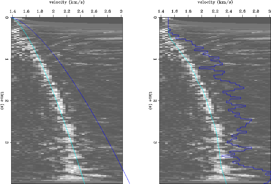
Figure ![[*]](http://sepwww.stanford.edu/latex2html/cross_ref_motif.gif) a demonstrates the initial parametric fit on a typical
semblance scan. The curve that lies closest to the semblance peaks is
the
a demonstrates the initial parametric fit on a typical
semblance scan. The curve that lies closest to the semblance peaks is
the ![]() curve given by (3) evaluated at the
curve given by (3) evaluated at the ![]() which maximize semblance. The smooth curve of higher average velocity
is the parametric interval velocity curve vi given by (4)
evaluated at
which maximize semblance. The smooth curve of higher average velocity
is the parametric interval velocity curve vi given by (4)
evaluated at ![]() .
.
The implementation of the parametric velocity search is diagrammed below:
INITIAL PARAMETRIC VELOCITY ESTIMATE
====================================
	* Choose parametric form:  Vrms = Vo + a * t**b
		- Vo = Vrms(t=0)
		- a   vertical velocity gradient
		- b   velocity "curvature"

1.4 <  Vo  < 1.6
			0.0 <   a  < 1.0
			0.0 <   b  < 2.0
	* Exhaustive search over finite parameter domain {Vo,a,b}
	* Retain Vrms*(Vo*,a*,b*) that maximizes semblance
	* Vrms* -> Vint*  is analytic
	* RESULT:
		- a Vrms* parametric fit that is globally "optimal"
		- a Vint* model that is physically reasonable
		- a starting point for MC random walks and constraints
The parametric fit in Figure ![[*]](http://sepwww.stanford.edu/latex2html/cross_ref_motif.gif) a seems remarkably reasonable.
The amount of velocity misfit is subtle compared to the Monte Carlo
fit shown in Figure
a seems remarkably reasonable.
The amount of velocity misfit is subtle compared to the Monte Carlo
fit shown in Figure ![[*]](http://sepwww.stanford.edu/latex2html/cross_ref_motif.gif) b. This can be seen by examining a
section stacked with parametric
b. This can be seen by examining a
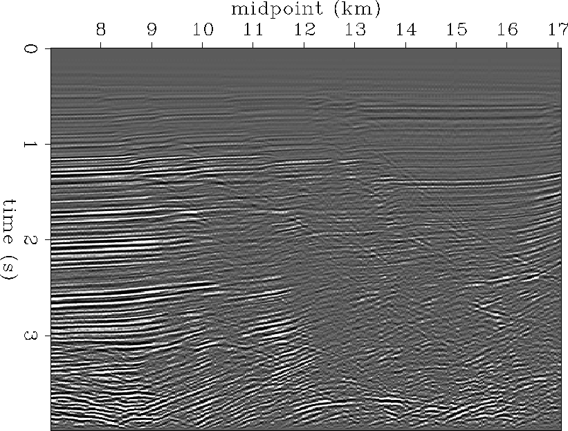
section stacked with parametric ![]() velocities. Figure
velocities. Figure ![[*]](http://sepwww.stanford.edu/latex2html/cross_ref_motif.gif) shows a section stacked with a 1-D velocity function, which is an
optimal Monte Carlo fit at midpoint 7 km. Figure
shows a section stacked with a 1-D velocity function, which is an
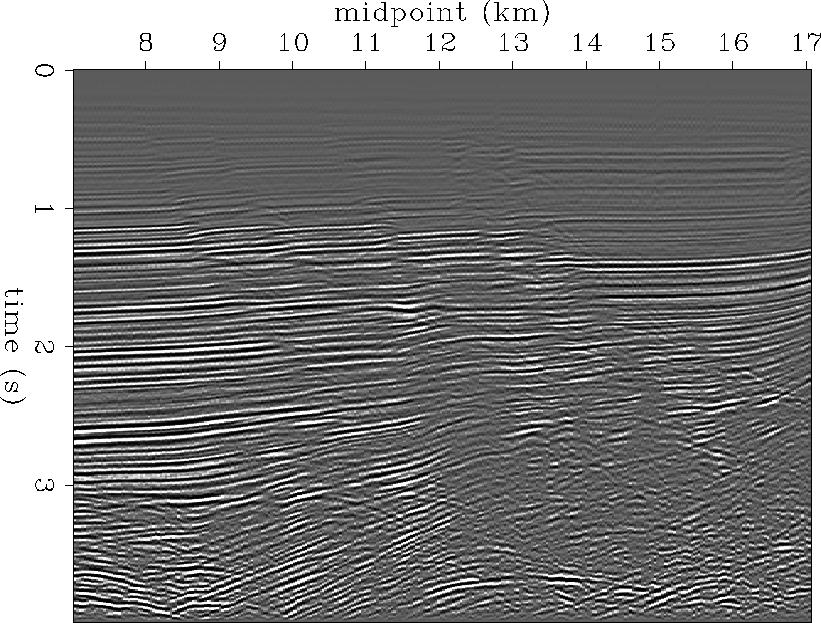
optimal Monte Carlo fit at midpoint 7 km. Figure ![[*]](http://sepwww.stanford.edu/latex2html/cross_ref_motif.gif) has
been stacked with the smoothed 2-D parametric velocity field.
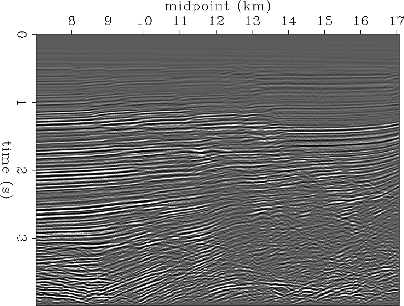
Figure
has
been stacked with the smoothed 2-D parametric velocity field.
Figure ![[*]](http://sepwww.stanford.edu/latex2html/cross_ref_motif.gif) is the optimal stack using the smoothed 2-D
Monte Carlo velocity picks, to be discussed in the next section.
is the optimal stack using the smoothed 2-D
Monte Carlo velocity picks, to be discussed in the next section.
The 1-D velocity stack in Figure ![[*]](http://sepwww.stanford.edu/latex2html/cross_ref_motif.gif) is coherent at the west where the
single Monte Carlo velocity analysis was done, but fades to the east
due to significant lateral velocity variation that is not accounted for
by the 1-D stacking velocity. The 2-D parametric velocity stack is
very coherent across the entire line in Figure
is coherent at the west where the
single Monte Carlo velocity analysis was done, but fades to the east
due to significant lateral velocity variation that is not accounted for
by the 1-D stacking velocity. The 2-D parametric velocity stack is
very coherent across the entire line in Figure ![[*]](http://sepwww.stanford.edu/latex2html/cross_ref_motif.gif) . Finally,
the 2-D Monte Carlo velocity stack is the best, as shown in Figure
. Finally,
the 2-D Monte Carlo velocity stack is the best, as shown in Figure
![[*]](http://sepwww.stanford.edu/latex2html/cross_ref_motif.gif) . The Monte Carlo stack is superior in its resolution of
shallow fault structure and fault diffractions, as well as
within the fault block at 12.5 km and 2 seconds depth. However,
for a ``quick and dirty velocity field,'' the parametric search
can be very fast and effective.
. The Monte Carlo stack is superior in its resolution of
shallow fault structure and fault diffractions, as well as
within the fault block at 12.5 km and 2 seconds depth. However,
for a ``quick and dirty velocity field,'' the parametric search
can be very fast and effective.
 |
 |
 |
 |