 |
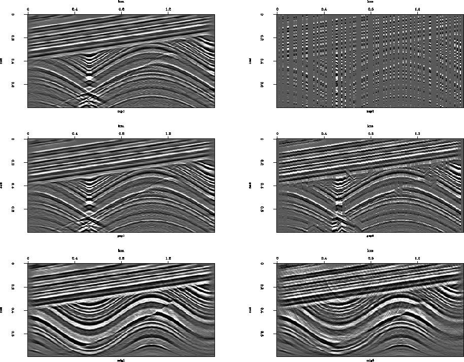
Figure 1 Top is data. Left is without gaps. Right is with gaps. Middle is linear interpolation over gaps. Bottom is migration.
 |
The top two frames of Figure 1
show the synthetic data I made for this study.
The synthetic data in Figure 1 is on a ![]() mesh.
The right frame shows the data with 150 of 200 channels deleted
by an algorithm that considers traces 4 at a time and then
randomly selects one to be kept while the other 3 are deleted.
The middle row of the figure shows that the method of
Claerbout
1992c
is not powerful enough to do a fully satisfactory job of
filling in the missing traces
because of the many smiles in migration shown in the bottom row.
My hypothesis is that
I should be able to improve the data interpolation
based on the concept that the migration on the bottom right
should have smiles removed by the principle
that the migration should leave a local monoplane
as described in Claerbout
1992d.
mesh.
The right frame shows the data with 150 of 200 channels deleted
by an algorithm that considers traces 4 at a time and then
randomly selects one to be kept while the other 3 are deleted.
The middle row of the figure shows that the method of
Claerbout
1992c
is not powerful enough to do a fully satisfactory job of
filling in the missing traces
because of the many smiles in migration shown in the bottom row.
My hypothesis is that
I should be able to improve the data interpolation
based on the concept that the migration on the bottom right
should have smiles removed by the principle
that the migration should leave a local monoplane
as described in Claerbout
1992d.
The number of missing data points is ![]() .The migration-diffraction program for the synthetic data
runs both ways in a few seconds.
Thus, theoretically, a linear least squares solution
for the unknowns should run in a day or two.
On the discouraging side,
the problem is not one of linear least squares,
and the code has not yet been written.
Nonlinear least squares arises because we must simultaneously
estimate the model covariance matrix.
On the encouraging side,
SEP has a parallel computer and the times quoted above
are for my desktop workstation.
Also, satisfactory results may be found
long before the theoretically required 30,000 iterations.
.The migration-diffraction program for the synthetic data
runs both ways in a few seconds.
Thus, theoretically, a linear least squares solution
for the unknowns should run in a day or two.
On the discouraging side,
the problem is not one of linear least squares,
and the code has not yet been written.
Nonlinear least squares arises because we must simultaneously
estimate the model covariance matrix.
On the encouraging side,
SEP has a parallel computer and the times quoted above
are for my desktop workstation.
Also, satisfactory results may be found
long before the theoretically required 30,000 iterations.
To be a success, I believe I should
achieve useful results in 100 or fewer iterations,
preferably in a handful of iterations.
Fundamentally, many issues arise.
Is a preconditioning strategy essential?
Damping is an important part of any inversion formulation.
Does damping speed the arrival of a useful solution?
Figure ![[*]](http://sepwww.stanford.edu/latex2html/cross_ref_motif.gif) suggests that
nearest-neighbor interpolations could frustrate
iterative migrations. Will it?
Is a conversion to the antialias method of
Claerbout (1992a) mandatory or advisable?
(That would require vectorizing that code over the midpoint axis,
a non-trivial undertaking.)
How can/should the covariance matrices be bootstrapped?
Because of this bewildering array of imponderables,
and because of my many frustrating experiences with
iterating least-squares problems of high dimensionality
Claerbout (1990) and others, unpublished,
I chose not to attack the problem frontally,
but begin by examining the ingredients to any inversion,
the gradient, the gradient after filtering with
the inverse-covariance filters, etc.
suggests that
nearest-neighbor interpolations could frustrate
iterative migrations. Will it?
Is a conversion to the antialias method of
Claerbout (1992a) mandatory or advisable?
(That would require vectorizing that code over the midpoint axis,
a non-trivial undertaking.)
How can/should the covariance matrices be bootstrapped?
Because of this bewildering array of imponderables,
and because of my many frustrating experiences with
iterating least-squares problems of high dimensionality
Claerbout (1990) and others, unpublished,
I chose not to attack the problem frontally,
but begin by examining the ingredients to any inversion,
the gradient, the gradient after filtering with
the inverse-covariance filters, etc.