Local windows

The earth dip changes rapidly with location. In a small region there is a local dip and dip bandwidth which determining the best LOMOPLAN (LOcal MOPLAN). To see how to cope with the edge effects of filtering in a small region, and to see how to patch together these small regions, see my article ().

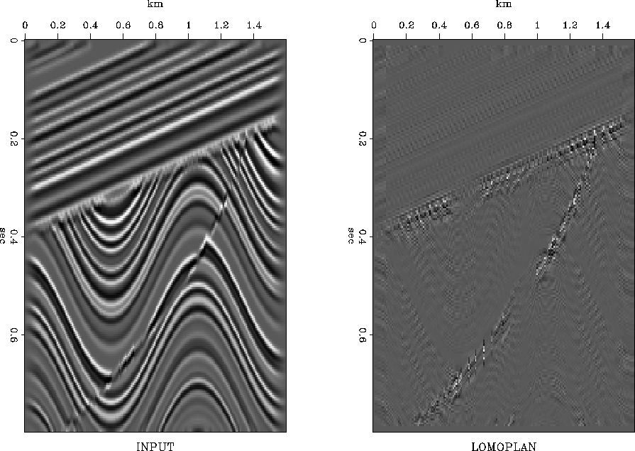
Figure 1 shows a synthetic model that illustrates local variation in bedding. Notice dipping bedding, curved bedding, unconformity between them, and a fault in the curved bedding. Also, notice the image has its amplitude tapered to zero on the left and right sides. After local monoplane annihilation (LOMOPLAN) the continuous bedding is essentially gone. The fault and unconformity remain.

 

sigmoid0
Figure 1 Left is a synthetic reflectivity model. Right is the result of local monoplane annihilation.

The local spatial prediction-error filters contain the essence of a factored form of the inverse covariance matrix of the model.

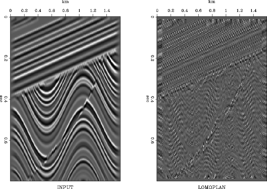
The local spatial prediction-error filters contain the essence of a factored form of the inverse covariance matrix of the model. A covariance matrix has two aspects: a spectral aspect in the prediction-error filter and an amplitude aspect as in gain leveling. Thus the final step in local whitening is to divide the filters by the amplitude of the filter output. This is like applying automatic gain adjustment to the residuals in Figure 1. Doing this gives Figure 2.

 

sigmoid1
Figure 2 Left is a synthetic reflectivity model. Right is the result of local monoplane annihilation with inverse amplitudes.

Notice the model weakens in amplitude along the sides. (The designer of this model (me) evidently planned to use the model for diffraction and migration.) These damping amplitudes are strong on the LOMOPLAN because a damping plane wave has angular bandwidth greater than zero. Two ways to go beyond the monoplane model are (1) to bend the plane, or (2) to allow amplitude variation along the plane. A one point filter will predict perfectly an exponentially growing or decaying amplitude along a plane wave. But I prefer a bad prediction of the damping plane as an indication that the planar model is breaking down. (Here I took a hint from one-dimensional filter analysis. Recall Burg's old ``forward and backward'' residual trick (FGDP, p. 134). By forcing a 1-D two-term filter to predict both backward and forward, Burg avoids perfect predictability on growing exponentials.) To achieve imperfect prediction of exponentially growing planes, I require one filter to extinguish two copies of the data, the original copy and a second copy with both $\tau$ and x reversed. Note that dips on the reversed copy are the same as on the original but amplitude growth on one is decay on the other. To give these ideas concrete form, I prepared subroutine burg2() which applies a convolution to both forward and reversed data.

# Burg2 -- Burg 2-D conv with (a1,a2) filter (monoplane annihilator if a2=2)
# 	output residual partitioned into normal and backward parts.
#	output conjugate to FILTER.
#	output residual(,) aligns with data(,) at filter coef aa(lag1,lag2)
#
subroutine burg2( conj,add, lag1,lag2, data,n1,n2,  aa,a1,a2,  residual)
integer i1,i2,    conj,add, lag1,lag2,      n1,n2,     a1,a2
real 				       data(n1,n2) ,aa(a1,a2), residual(n1,2*n2)
temporary real 			       back(n1,n2)
call conjnull(    conj,add,                         aa,a1*a2,  residual,n1*n2*2)
do i2= 1, n2 {
do i1= 1, n1 {	back( n1-i1+1, n2-i2+1) = data( i1, i2)
		}}
call cinlof( conj, 1, lag1,lag2, n1,n2,data, a1,a2,aa, residual        )
call cinlof( conj, 1, lag1,lag2, n1,n2,back, a1,a2,aa, residual(1,n2+1))
return;	end

To annihilate the best fitting plane, it is a simple matter of using subroutine burg2() in the conjugate-gradient context, as in PVI. This is done in subroutine moplan(). Notice the backward residual in residual( 1, n2+1...2*n2).

# mono plane annihilator and its residual
#
subroutine moplan( agc, eps, data,n1,n2, niter, lag1,lag2, gap, aa,a1,a2, rr)
integer            agc,           n1,n2, niter, lag1,lag2, gap,    a1,a2
real	dot, lam,       eps, data(n1,n2),            aa(a1,a2),rr(n1*n2*2+a1*a2)
integer	i1, a12, r12, iter
temporary real da( a1,a2),  dr( n1*n2*2+a1*a2)
temporary real sa( a1,a2),  sr( n1*n2*2+a1*a2)
a12 = a1 * a2;		r12 = n1 * n2 * 2
call null( rr, r12+a12);	call null( aa, a12);	aa( lag1, lag2 ) = 1.
call null( dr, r12+a12);	call null( da, a12)
call         burg2 ( 0, 0, lag1,lag2, data,n1,n2, aa,a1,a2, rr       )
                           lam =  eps * sqrt( dot( r12, rr, rr))
call         ident ( 0, 0, lam,     a12,          aa,       rr(r12+1))
call         scale (    -1.,    r12+a12,                    rr       )
do iter= 0, niter {
	call burg2 ( 1, 0, lag1,lag2, data,n1,n2, da,a1,a2, rr       )
	call ident ( 1, 1, lam,     a12,          da,       rr(r12+1))

do i1= 1, min0( a1, lag1+gap-1) {         da(i1,lag2)= 0.}
	call burg2 ( 0, 0, lag1,lag2, data,n1,n2, da,a1,a2, dr       )
	call ident ( 0, 0, lam,     a12,          da,       dr(r12+1))
	call cgstep( iter,  a12 , aa,da,sa,
			a12+r12 , rr,dr,sr )
	}
if( agc>0)   call scale( 1./sqrt(dot(r12,rr,rr)), a1*a2,aa)
call 	     burg2 ( 0, 0, lag1,lag2, data,n1,n2, aa,a1,a2, rr)
return; end

As an afterthought, moplan() also offers the agc option, inverse scaling by the RMS value.