

Next: Computation of the conjugate
Up: FINITE DIFFERENCE METHODS
Previous: Computation of matrix
The gradient vector defined in equation (5) is the sum of
traveltime residual term  and
condition term
  . The computation of the
condition term is straightforward because matrix
  is given.
In principle, we can compute the traveltime residual term by first computing
matrix
  , and then performing the matrix multiplication.
However, matrix
  has
has  elements that are functions of r;
hence, both its calculation and storage are of high cost. If we can compute
the vector
  directly using a finite difference method, we can
considerably reduce the cost in computation time and storage.
If we solve the first-order linear PDE (9)
using the method of characteristics, we find that
|  |
(10) |
where  and
and  are
the coordinates of the ray that starts
from the number i source and ends at the receiver at depth r, and s is
the arc-length of the ray. Clearly, the elements of matrix
  are
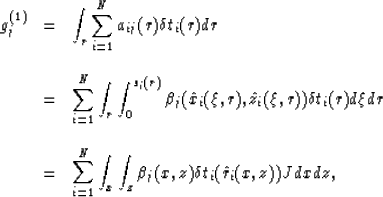
the integrations of the basis functions along rays. The component of the
gradient vector can be computed as follows:
|  |
(11) |
where J is the Jacobian of the coordinate transformation:
|  |
(12) |
The last step of equation (11) is an area integration that
is easy to implement. Appendix A shows
that function  satisfies the first-order
linear PDE, as follows:
|  |
(13) |
with the initial condition that function  is equal to the
receiver depth at each receiver location. We can use a finite difference
algorithm, similar to the one used for traveltime calculation, to solve
equation (13). The algorithm should start from receiver locations,
and extrapolate function
  in the opposite directions of
the wave propagations, towards the source.


Next: Computation of the conjugate
Up: FINITE DIFFERENCE METHODS
Previous: Computation of matrix
Stanford Exploration Project
12/18/1997
![]() and
condition term
and
condition term ![]() . The computation of the
condition term is straightforward because matrix
. The computation of the
condition term is straightforward because matrix ![]() is given.
In principle, we can compute the traveltime residual term by first computing
matrix
is given.
In principle, we can compute the traveltime residual term by first computing
matrix ![]() , and then performing the matrix multiplication.
However, matrix
, and then performing the matrix multiplication.
However, matrix ![]() has
has ![]() elements that are functions of r;
hence, both its calculation and storage are of high cost. If we can compute
the vector
elements that are functions of r;
hence, both its calculation and storage are of high cost. If we can compute
the vector ![]() directly using a finite difference method, we can
considerably reduce the cost in computation time and storage.
directly using a finite difference method, we can
considerably reduce the cost in computation time and storage.

