

Next: CONCLUSIONS
Up: Cunha: Elastic Migration
Previous: Computation of the local
A synthetic dataset comprising a hundred shot gathers was generated
with the modeling scheme described in Cunha (1991). The model includes
isotropic and transverse isotropic layers, which are described at
each point by five parameters (c11, c33, c13, c55, and  ).
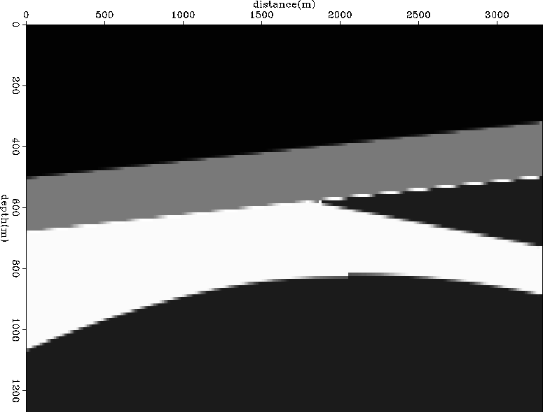
Figure
 ![[*]](http://sepwww.stanford.edu/latex2html/cross_ref_motif.gif) shows the c11 component of the model, while
Figure
shows the c11 component of the model, while
Figure ![[*]](http://sepwww.stanford.edu/latex2html/cross_ref_motif.gif) shows the 2 components of the recorded wavefield for one shot.
shows the 2 components of the recorded wavefield for one shot.
syntmodel
Figure 2 The c11 stiffness component of the synthetic structural model used to
generate the data of Figure ![[*]](http://sepwww.stanford.edu/latex2html/cross_ref_motif.gif) . The model includes
isotropic and transverse isotropic layers.
. The model includes
isotropic and transverse isotropic layers.


 dataslice
Figure 3 One of the synthetic shot records generated by finite differences elastic
modeling. (a) Is the vertical component of the displacement
field recorded at the surface. (b) Is the
horizontal component of the same field. The relative weakness of the shallow
reflection at large offsets is caused by the introduction of a thin absorbing
region near the free surface in order to simulate a low Q, unconsolidated
sediment. Click the button to see a movie with every tenth shot gather.
The first set is the z component and the second set is the x component.


A migrated shot gather and the result of stacking all the migrated
shot gathers are shown in Figure ![[*]](http://sepwww.stanford.edu/latex2html/cross_ref_motif.gif) . The low resolution
around the horizontal position of 2000 meters was caused by the
accidental missing of twenty consecutives migrated shot gathers,
sufficiently close to the report dead line.
The acquisition geometry was off-end, with receivers at the right
of the source.
. The low resolution
around the horizontal position of 2000 meters was caused by the
accidental missing of twenty consecutives migrated shot gathers,
sufficiently close to the report dead line.
The acquisition geometry was off-end, with receivers at the right
of the source.
migimag
Figure 4 (a) Migrated image of one shot gather. (b) Stacking
of the migrated shot gathers.The interfaces of the correct model
are overlaid to the stacked session.


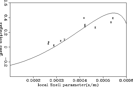
The retrieved angle-dependent reflectivity at one of the
reflectors is compared in Figure ![[*]](http://sepwww.stanford.edu/latex2html/cross_ref_motif.gif) to the theoretical
reflectivity function. Although the retrieved reflectivity function
fits the general trend of the theoretical curve, it is clear that the
method still needs some refinement to allow its application to real data.
to the theoretical
reflectivity function. Although the retrieved reflectivity function
fits the general trend of the theoretical curve, it is clear that the
method still needs some refinement to allow its application to real data.
refofp
Figure 5 The X represent the retrieved reflectivity as a function of the
local Snell parameter and the continuous line, the theoretical reflectivity
function


Next: CONCLUSIONS
Up: Cunha: Elastic Migration
Previous: Computation of the local
Stanford Exploration Project
12/18/1997
![[*]](http://sepwww.stanford.edu/latex2html/cross_ref_motif.gif) shows the c11 component of the model, while
Figure
shows the c11 component of the model, while
Figure ![[*]](http://sepwww.stanford.edu/latex2html/cross_ref_motif.gif) shows the 2 components of the recorded wavefield for one shot.
shows the 2 components of the recorded wavefield for one shot.
![]() ).
Figure
).
Figure ![[*]](http://sepwww.stanford.edu/latex2html/cross_ref_motif.gif) shows the c11 component of the model, while
Figure
shows the c11 component of the model, while
Figure ![[*]](http://sepwww.stanford.edu/latex2html/cross_ref_motif.gif) shows the 2 components of the recorded wavefield for one shot.
shows the 2 components of the recorded wavefield for one shot.

![[*]](http://sepwww.stanford.edu/latex2html/cross_ref_motif.gif) . The model includes
isotropic and transverse isotropic layers.
. The model includes
isotropic and transverse isotropic layers.

![[*]](http://sepwww.stanford.edu/latex2html/cross_ref_motif.gif) . The low resolution
around the horizontal position of 2000 meters was caused by the
accidental missing of twenty consecutives migrated shot gathers,
sufficiently close to the report dead line.
The acquisition geometry was off-end, with receivers at the right
of the source.
. The low resolution
around the horizontal position of 2000 meters was caused by the
accidental missing of twenty consecutives migrated shot gathers,
sufficiently close to the report dead line.
The acquisition geometry was off-end, with receivers at the right
of the source.

![[*]](http://sepwww.stanford.edu/latex2html/cross_ref_motif.gif) to the theoretical
reflectivity function. Although the retrieved reflectivity function
fits the general trend of the theoretical curve, it is clear that the
method still needs some refinement to allow its application to real data.
to the theoretical
reflectivity function. Although the retrieved reflectivity function
fits the general trend of the theoretical curve, it is clear that the
method still needs some refinement to allow its application to real data.
