

Next: Conclusions
Up: Karrenbach: Prestack reverse-time migration
Previous: SYNTHETIC EXAMPLE WITH TRANSVERSE
The above outlined algorithm is implemented on the Connection Machine.
Finite-differences algorithms are very well suited to
massively parallel
computers, since the computational grid exactly maps onto the
layout of processors.
I found that my code ran at about 113 Mflops on a 4K machine.
The algorithm could be much faster, if it were not for the boundary conditions,
which are used to prevent reflections from the side and bottom boundaries.
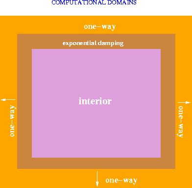
Using a one-way wave equation with absorbing boundaries necessitates the use of
different finite-difference stencils in the interior and at various locations
at the boundary.
domains
Figure 2 The computational domain in this implementation is divided into three parts: interior, exponential-damping boundary and one-way wave equation absorbing boundaries. In each of those domains different finite difference operators can vary in form domain to domain. An elegant solution is to have a super-stencil, so that the same stencil can be used in all domains. This implies some computational overhead and increased memory use.
|
|  |

If the memory of the machine is big enough, an efficient implementation
is possible, where spatially variable finite-difference coefficients are used.
The shape of the stencil is constant over the entire grid.
Using the SEP machine, which has small memory, I could not apply this elegant
approach efficiently, since I would have had to
truncate my problem size unrealistically.
I really liked to use the Connection Machine as a movie program, seeing
wave propagation snapshots as they are calculated. This instant
feedback makes the machine useful as a teaching tool.
Zxseis
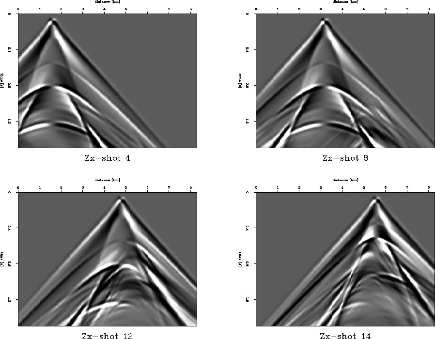
Figure 3 Shot gather generated by a vertical source and horizontal inline receiver.
 Zzseis
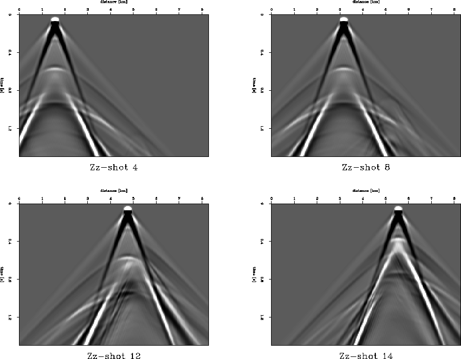
Figure 4 Shot gather generated by a vertical source and vertical receiver.
 Xxseis
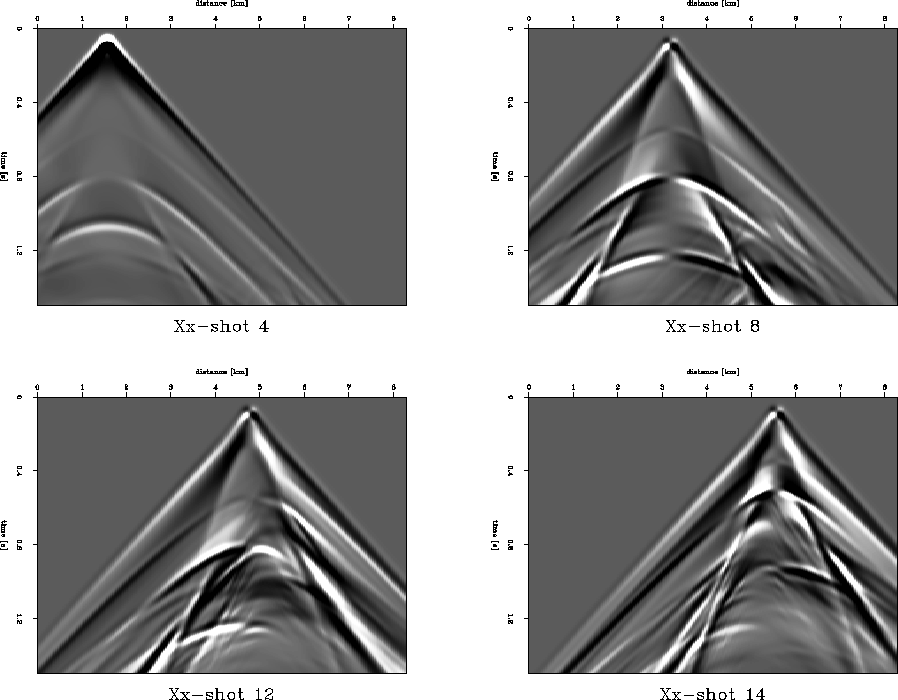
Figure 5 Shot gather generated by a horizontal inline source and a horizontal inline receiver.
 Xzseis
Figure 6 Shot gather generated by a horizontal inline source and a vertical receiver.
 zimagestack
Figure 7 Elastic stiffnesses imaged using 16 shots. Source vector was vertical.
 ximagestack
Figure 8 Elastic stiffnesses imaged using 16 shots. Source vector was vertical.


Next: Conclusions
Up: Karrenbach: Prestack reverse-time migration
Previous: SYNTHETIC EXAMPLE WITH TRANSVERSE
Stanford Exploration Project
12/18/1997
