


To create a 2-D velocity model from sonic logs, one needs to do interpolation. Wells are often drilled with large separating distances. Data collected with such a large sample interval are often believed to be seriously aliased. Is it possible to interpolate this kind of data? The answer is positive if we are interested in having a smooth 2-D velocity model. Because smooth sonic logs are non-Gaussian, they can be interpolated with a non-linear method.
The next question one may ask is how the interpolation should be done. My idea is that this kind of data should be interpolated along its contour lines because data samples along these trajectories have constant values. Based on this idea, I developed a two-step algorithm to interpolate this kind of data. First, I use the known well logs to predict the contour lines of data. Then I interpolate data along these contour lines. Predicting contour lines for such sparsely sampled data is an underdetermined problem. I use a model to parameterize the contour lines. If only two well logs are available, the contour lines are straight lines. If three or more well logs are available, then the contour lines are modeled by cubic-spline functions. These models are parameterized by the depth positions of the contour lines at the locations of the known wells. Once we find these depth positions, we can generate the whole set of contour lines.
Suppose a contour has a depth position z at well 1 and a depth
position ![]() at well 2. Then the log sample u1(z)
at well 1 should be equal to the log sample
at well 2. Then the log sample u1(z)
at well 1 should be equal to the log sample ![]() because they are on the same contour line. Therefore, we can estimate
because they are on the same contour line. Therefore, we can estimate ![]() by minimizing the difference between u1(z) and
by minimizing the difference between u1(z) and ![]() .Obviously,
.Obviously, ![]() is a function of z. We can estimate the function
is a function of z. We can estimate the function
![]() through the constrained non-linear optimization as we did
for dip estimation. The constraint for this problem is that
the contour lines do not cross each other. When three or more
well logs are available,
through the constrained non-linear optimization as we did
for dip estimation. The constraint for this problem is that
the contour lines do not cross each other. When three or more
well logs are available, ![]() is estimated for each pair of
well logs. From these functions, I generate all contour lines and interpolate
data along these contour lines.
is estimated for each pair of
well logs. From these functions, I generate all contour lines and interpolate
data along these contour lines.
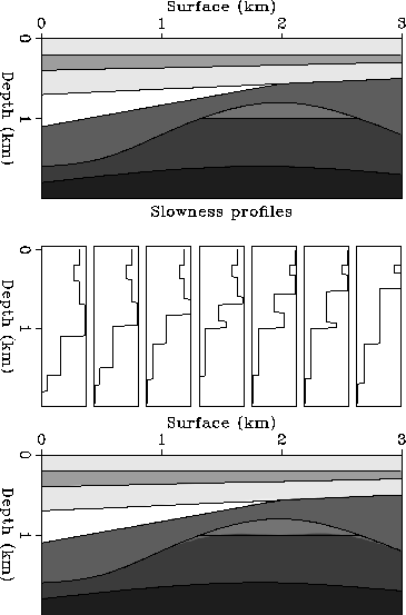
I used a synthetic model to test my interpolation algorithm. The top
panel of Figure ![[*]](http://sepwww.stanford.edu/latex2html/cross_ref_motif.gif) shows a synthetic slowness model. The
model has fairly complicated subsurface structure. The interval slowness
within each layer is constant. The middle panel of the
figure shows seven slowness profiles that simulates the well logs
measured from the synthetic model and with a large separating distance.
The bottom panel of Figure displays the slowness model
interpolated from those slowness profiles. The interfaces of the original model
are plotted on the same panel. The algorithm
does a very good job. The interpolated model is very close to the original
model except at the pinch-out.
shows a synthetic slowness model. The
model has fairly complicated subsurface structure. The interval slowness
within each layer is constant. The middle panel of the
figure shows seven slowness profiles that simulates the well logs
measured from the synthetic model and with a large separating distance.
The bottom panel of Figure displays the slowness model
interpolated from those slowness profiles. The interfaces of the original model
are plotted on the same panel. The algorithm
does a very good job. The interpolated model is very close to the original
model except at the pinch-out.
 |

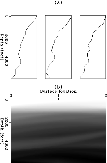
Now I show some field data examples. Figure a displays
three smoothed sonic logs. The distances
between wells are several kilometers. Figure b shows the
result of interpolation. The interpolated model is smooth. It has
a well-defined high velocity layer at depth of 3 km and a well-defined
low velocity layer at the depth of 4 km. Unfortunately, I am not able to
check the accuracy of this result.
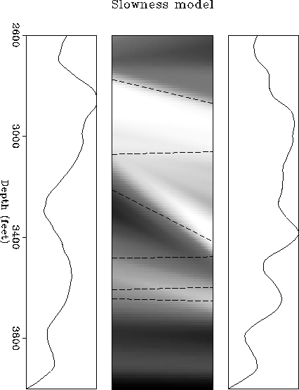
The well logs shown in Figure are collected from two wells
between which a cross-well experiment was conducted. The middle panel
of this figure displays the interpolated slowness model. The dashed lines
on this panel are the geological structures interpreted from
an independent source (Harris et al., 1990). It is clear that the two
results agree fairly well.
 |
 |