

Next: Results
Up: A REAL DATA EXAMPLE
Previous: A REAL DATA EXAMPLE
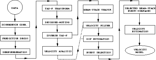
Figure ![[*]](http://sepwww.stanford.edu/latex2html/cross_ref_motif.gif) shows the processing sequence applied to
the data to alleviate the influence of noise and event-crossing
in the velocity inversion.
Although muting could be used to eliminate event-crossing, this would
result in the discharge of useful information from a particularly
important part of the reflections. Multiples and other coherent
noise were attenuated by filtering techniques while the
problem of interference between reflections was solved by
a differential treatment of the shallow reflections.
shows the processing sequence applied to
the data to alleviate the influence of noise and event-crossing
in the velocity inversion.
Although muting could be used to eliminate event-crossing, this would
result in the discharge of useful information from a particularly
important part of the reflections. Multiples and other coherent
noise were attenuated by filtering techniques while the
problem of interference between reflections was solved by
a differential treatment of the shallow reflections.
flux
Figure 8 The processing sequence applied to the marine data shown in
Figure ![[*]](http://sepwww.stanford.edu/latex2html/cross_ref_motif.gif) a.
a.

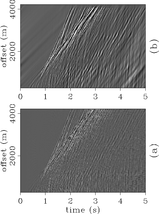
It is clear from Figure ![[*]](http://sepwww.stanford.edu/latex2html/cross_ref_motif.gif) a that despite the application
of predictive deconvolution and a dereverberation algorithm
(described in Cunha and Muir, 1989), complex
multiples and peg-legs are still dominant features in the data.
More effective in the elimination of the multiples and linear
noises was the application of a filter in the
a that despite the application
of predictive deconvolution and a dereverberation algorithm
(described in Cunha and Muir, 1989), complex
multiples and peg-legs are still dominant features in the data.
More effective in the elimination of the multiples and linear
noises was the application of a filter in the  domain.
The direct and inverse
  transform were performed by
an algorithm developed by Kostov (1989); Figure
 ![[*]](http://sepwww.stanford.edu/latex2html/cross_ref_motif.gif) a
shows the shape of the cutoff curve.
The high-slowness part of the shallow reflections is located
inside the rejecting region to avoid the reflections interfering
in the subsequent processing of the reflections below them.
Figure
a
shows the shape of the cutoff curve.
The high-slowness part of the shallow reflections is located
inside the rejecting region to avoid the reflections interfering
in the subsequent processing of the reflections below them.
Figure ![[*]](http://sepwww.stanford.edu/latex2html/cross_ref_motif.gif) b shows the filtered data transformed back to
the x-t domain.
b shows the filtered data transformed back to
the x-t domain.
cmps
Figure 9 (a) CMP gather from Brazil offshore after deconvolution
and dereverberation.
(b) The same data after filtering in the  domain.
 taupbeam
Figure 10 (a) The shape of cutoff curve used in the  domain filter.
The bandpass region lies at the left side of the curve. (b)
A surface slice of the filtered beam-stack cube along the 8th event.
The overlaid curve corresponds to the mapping of the velocity-cutoff
curve of Figure
domain filter.
The bandpass region lies at the left side of the curve. (b)
A surface slice of the filtered beam-stack cube along the 8th event.
The overlaid curve corresponds to the mapping of the velocity-cutoff
curve of Figure![[*]](http://sepwww.stanford.edu/latex2html/cross_ref_motif.gif) b into this domain.
The transition between the pass (to the left of the curve) and cut
(to the right of the curve) regions is actually smooth.
b into this domain.
The transition between the pass (to the left of the curve) and cut
(to the right of the curve) regions is actually smooth.

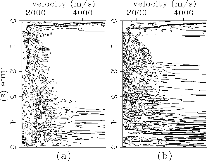
A comparison between the velocity spectra of the data before
and after the  filtering (Figure
 ![[*]](http://sepwww.stanford.edu/latex2html/cross_ref_motif.gif) ) shows a
good improvement in the resolution of primary events after the
filtering. The times of the picks associated with primaries were
used as the starting points for the event-detection algorithm.
The dashed line in Figure
) shows a
good improvement in the resolution of primary events after the
filtering. The times of the picks associated with primaries were
used as the starting points for the event-detection algorithm.
The dashed line in Figure ![[*]](http://sepwww.stanford.edu/latex2html/cross_ref_motif.gif) b defines the cutoff
velocity function for the velocity filter that was applied to
the beam-stacked data. The application of this filter is
essential to avoid the interference of multiples, not only
in the event-picking algorithm, but also in the final
inversion step.
b defines the cutoff
velocity function for the velocity filter that was applied to
the beam-stacked data. The application of this filter is
essential to avoid the interference of multiples, not only
in the event-picking algorithm, but also in the final
inversion step.
A total of sixteen events were selected for the inversion.
Their a priori nearest-offset times were selected from
the velocity spectrum, but the event-picking algorithm had a
pre-specified degree of freedom to reestimate them.
The four initial events (which cross the reflections below)
were selected with the help of a normal-moveout overlay
program (Claerbout, 1987).
The last step before the velocity estimation algorithm
selects the slices along the event-mapped
surfaces in the beam-stack cube (Figure ![[*]](http://sepwww.stanford.edu/latex2html/cross_ref_motif.gif) b).
The slices corresponding to
the shallow events are taken from a non-[
b).
The slices corresponding to
the shallow events are taken from a non-[ ]filtered
version of the beam-stack cube.
To optimize the estimation, the beam-stack of the shallow events (1 to 9)
was computed apart from the deep events (9 to 16), so that a
lower slowness interval could be used for the latter.
velans
Figure 11 Velocity spectrum of (a) the deconvolved data, and (b)
the same data after the  filtering. The dashed line represents
the cutoff curve used in the velocity-filter applied to the beam-stack.


Next: Results
Up: A REAL DATA EXAMPLE
Previous: A REAL DATA EXAMPLE
Stanford Exploration Project
12/18/1997
![[*]](http://sepwww.stanford.edu/latex2html/cross_ref_motif.gif) shows the processing sequence applied to
the data to alleviate the influence of noise and event-crossing
in the velocity inversion.
Although muting could be used to eliminate event-crossing, this would
result in the discharge of useful information from a particularly
important part of the reflections. Multiples and other coherent
noise were attenuated by filtering techniques while the
problem of interference between reflections was solved by
a differential treatment of the shallow reflections.
shows the processing sequence applied to
the data to alleviate the influence of noise and event-crossing
in the velocity inversion.
Although muting could be used to eliminate event-crossing, this would
result in the discharge of useful information from a particularly
important part of the reflections. Multiples and other coherent
noise were attenuated by filtering techniques while the
problem of interference between reflections was solved by
a differential treatment of the shallow reflections.


