To avoid the problems arising from the poor estimation of p
in the picked-based method, I devised a hybrid algorithm, in which
the events are still defined through the picking process, but
instead of estimating horizontal slownesses, this algorithm uses
a probability distribution ![]() which is computed
for each event by using beam-stacks.
which is computed
for each event by using beam-stacks.
Beam-stacks represent a mapping of the x-t plane onto the p-x-t cube ( Biondi, 1990). For each point (x,t) in the object plane a sum is performed over a finite path, centered at that point and parametrized by p, with the result corresponding to the point (p,x,t) in the image cube. Different transforms can be defined depending on the aperture of path (number of points in the sum) and the specific choice of parametric curve: slant-stack ("infinite" aperture) and local slant-stack (finite aperture) for a straight-line path, parabolic-transform for an "infinite" aperture parabolic path, and so on.
The concept of beam-stacks can be generalized to include semblance as well as stacking as the basic transform operation. Biondi (1990) compared the semblance spectrum obtained with straight, parabolic, and hyperbolic finite aperture curves. His results indicated that the hyperbolic-stack has a superior resolution power.
In the hybrid scheme, we interpret the hyperbolic semblance spectrum
![]() as the (non normalized) probability that a given point x
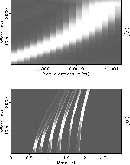
of event j have a horizontal slowness p. Figure
as the (non normalized) probability that a given point x
of event j have a horizontal slowness p. Figure ![[*]](http://sepwww.stanford.edu/latex2html/cross_ref_motif.gif) a
shows one plane of the three-dimensional beam-stack of the
synthetic data, and Figure
a
shows one plane of the three-dimensional beam-stack of the
synthetic data, and Figure ![[*]](http://sepwww.stanford.edu/latex2html/cross_ref_motif.gif) b shows
the two-dimensional beam-stack
b shows
the two-dimensional beam-stack ![]() corresponding to the
second event (
corresponding to the
second event (![]() sec.) of the same data.
sec.) of the same data.
 |
![[*]](http://sepwww.stanford.edu/latex2html/cross_ref_motif.gif) for p=0.17 msec/meter and
(b) a cut in the same beam-stack along the second
event of that data.
for p=0.17 msec/meter and
(b) a cut in the same beam-stack along the second
event of that data.
For a given p, v, and a point xj of reflection j equation 1 can be used to define the related point xj-1 in the reflection above (j-1) which share the same horizontal slowness
xj-1 = f(xj,p,v).
I define the function| |
(4) |
If the velocity is the true velocity, there will be one (and
only one) point xj for each value of p, for which
![]() will assume its maximum value (2.0). If the velocity
is not the true velocity,
will assume its maximum value (2.0). If the velocity
is not the true velocity, ![]() will not assume its
maximum value for all ps. Based on this assumption I
define
will not assume its
maximum value for all ps. Based on this assumption I
define
 |
(5) |
| |
(6) |
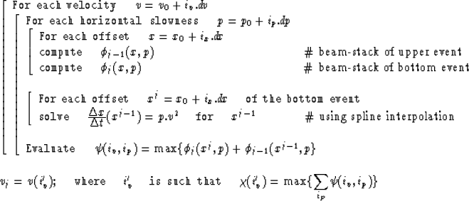
Differently from the picked-based method, the hybrid scheme requires the introduction of a scanning through a set of discretized velocities. For each pair of adjacent reflection events, the interval velocity is estimated by the following procedure:

The estimated velocity vj corresponds to the interval velocity
between reflectors ![]() and
and ![]() . Instead of repeating this
procedure for all pairs of adjacent reflectors, the actual
algorithm has an internal loop in
. Instead of repeating this
procedure for all pairs of adjacent reflectors, the actual
algorithm has an internal loop in ![]() that make it more
computationally efficient. Also, the beam-stacks are computed
only once, before the loop in v. Figure
that make it more
computationally efficient. Also, the beam-stacks are computed
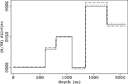
only once, before the loop in v. Figure ![[*]](http://sepwww.stanford.edu/latex2html/cross_ref_motif.gif) compares the
true model with the results of two inversion algorithms: one (dashed
line in the figure) finds the interval velocity model whose
Dix's related hyperbolas best fit the picked events; the other (dotted
line in the figure) is the result from the hybrid scheme inversion.
The first thing we observe in this figure is that the velocities
estimated by the hybrid scheme fits better the true model than both
the Dix's fitting and the purely picking-based scheme.
Most important, the error in the hybrid-method estimation does not
change with depth and, actually, is of the same order as the velocity
discretization interval (dv) used for the inversion.
compares the
true model with the results of two inversion algorithms: one (dashed
line in the figure) finds the interval velocity model whose
Dix's related hyperbolas best fit the picked events; the other (dotted
line in the figure) is the result from the hybrid scheme inversion.
The first thing we observe in this figure is that the velocities
estimated by the hybrid scheme fits better the true model than both
the Dix's fitting and the purely picking-based scheme.
Most important, the error in the hybrid-method estimation does not
change with depth and, actually, is of the same order as the velocity
discretization interval (dv) used for the inversion.
 |
![[*]](http://sepwww.stanford.edu/latex2html/cross_ref_motif.gif) ;
the dashed line represents the velocity model estimated Dix's
least squares fitting of the picked events; and
the dotted line represents the velocity model
obtained with the hybrid method.
;
the dashed line represents the velocity model estimated Dix's
least squares fitting of the picked events; and
the dotted line represents the velocity model
obtained with the hybrid method.