


As is well known, any solution ![]() of the
equation (30) in case of point source can be expressed in the
form
of the
equation (30) in case of point source can be expressed in the
form
| |
(39) |
Fundamental solution is a response of a medium to the
![]() -function as the source. It is easily understood
that (in case of piecewise smooth media with restricted numbers
of interfaces)
-function as the source. It is easily understood
that (in case of piecewise smooth media with restricted numbers
of interfaces) ![]() consists of some
singularities (discontinuities) that propagates with
correspondence to eiconal's equation (31) and relations
(32) and some very smooth field
consists of some
singularities (discontinuities) that propagates with
correspondence to eiconal's equation (31) and relations
(32) and some very smooth field ![]() .
.
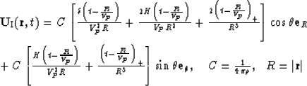
Let us consider a very simple example: a fundamental solution
that corresponds to a point vertical force in a homogeneous
medium (Figure ![[*]](http://sepwww.stanford.edu/latex2html/cross_ref_motif.gif) ) is
) is
| |
(40) |
 |
||
![\begin{eqnarraystar}
{\bf U}_{\rm II}( {\bf r}, t ) & = & -C \left[
{\delta \le...
...over V_s} \right )_+ \over R^3}
\right]
\cos \theta {\bf e}_R.\end{eqnarraystar}](img246.gif) |
||
shows radial (a) and angular (b)
component for some distance R and direction Let us perform the convolution in equation (39), bearing in mind that
| f(t)*Rq(t) = Iq f(t) = fq(t) | (41) |
Let ![]() be the observed field
(
be the observed field
(![]() or
or ![]() )
that is given on the surface of observation
)
that is given on the surface of observation
![]() and
and ![]() is a linear operator that transforms the
function
is a linear operator that transforms the
function ![]() into the field
into the field ![]() in the adjacent
domain
in the adjacent
domain ![]()
![]()
The action of the operator ![]() depends on the choice of the
function
depends on the choice of the
function ![]() which in turn
is a parameter in a fixed eikonal equation
which in turn
is a parameter in a fixed eikonal equation
| |
(42) |
![]()
![]()
We don't demand that the eikonal equation (42) is a characteristic equation of some hyperbolic differential operator. It is given, that's all!
Let us suppose that the field ![]() contains a
discontinuity
contains a
discontinuity ![]() (of some order q) with a travel time curve
(of some order q) with a travel time curve ![]() .It means that in a neighborhood of the surface
.It means that in a neighborhood of the surface
![]()
![]()
Generally speaking then, the wave field ![]() will contain one or
several discontinuities (with orders not necessarily equal to q)
and at least one of them will coincide with
will contain one or
several discontinuities (with orders not necessarily equal to q)
and at least one of them will coincide with ![]() at
at ![]() .If the position of this discontinuity is described by a
function
.If the position of this discontinuity is described by a
function ![]() , then
, then
| |
(43) |
We shall call the operator ![]() a kinematically-equivalent
operator of wave field continuation (on short K-operator, KO) if
the field
a kinematically-equivalent
operator of wave field continuation (on short K-operator, KO) if
the field ![]() necessarily contains at least one
discontinuity with eikonal
necessarily contains at least one
discontinuity with eikonal ![]() , that satisfies
equations (42) and (43) simultaneously.
, that satisfies
equations (42) and (43) simultaneously.
The notion of K-operator may be expanded to the case when both
fields ![]() and
and ![]() are vectorial fields.
In that case we have two equations (isotropic case) or three
equations (anisotropic case):
are vectorial fields.
In that case we have two equations (isotropic case) or three
equations (anisotropic case):
| |
(44) |
The question of existence of a K-operator corresponding to a given equation (42) can be simply answered (in a positive sense) if equation (42) is a characteristic equation for some equation in partial derivatives:
| |
(45) |
Let us consider the boundary value problem for equation (45) with condition
| |
(46) |
| |
(47) |
It is obvious that the solution contains at least one discontinuity
which at ![]() coincides
with
coincides
with ![]() and propagates with the eikonal
satisfying equation (42).
and propagates with the eikonal
satisfying equation (42).
Later we shall show that KO exists for any equation (42) if there
is a solution for the Cauchy problem for equation (42) with
the initial condition (43).
As a matter of fact there is a whole family ![]() of
K-operators that corresponds to the particular eikonal equation (42).
of
K-operators that corresponds to the particular eikonal equation (42).
K-equivalence is a notion which is much wider than
q-equivalence or (k)-equivalence. For instance, if ![]() belong to the same family
belong to the same family ![]() , then it is not
necessary that
, then it is not
necessary that
![]()
Let us consider K-operators for the classical eikonal equation
| |
(48) |
| |
(49) |
![]()
| |
(50) |
In order to get a unique solution of the equation (50) it is
necessary (and sufficient) to have a definite value
![]() in a starting point
in a starting point ![]() .We can express the vector
.We can express the vector ![]() in the form of a sum
in the form of a sum
![]()
![]()
Let us consider the case when ![]() is a curved surface and x and
y are a curvilinear system of coordinates. We propose that the axis
z coincides with the direction of a vector
is a curved surface and x and
y are a curvilinear system of coordinates. We propose that the axis
z coincides with the direction of a vector ![]() .
Let us determine a tangent plane P to
.
Let us determine a tangent plane P to ![]() in
the point
in
the point ![]() and let's introduce
the rectangular coordinates
and let's introduce
the rectangular coordinates ![]() and
and ![]() in P, then
in P, then
![]()
![]()
![]()
![]()
![]()
![]()
![]()
We have obtained that
![]()
).
It is easily understood that ![]() where
where
![]() is the time of propagation
from
is the time of propagation
from ![]() to
to ![]() .We shall call K-operator
.We shall call K-operator ![]() as the K-operator of forward (reverse)
wave field continuation and denote it as
as the K-operator of forward (reverse)
wave field continuation and denote it as ![]() (similarly
(similarly
![]() ) if in the neighbourhood of
) if in the neighbourhood of ![]() the field
the field
![]()
Each operator ![]() can be used for determination of the operator
can be used for determination of the operator ![]()
| |
(51) |
![]()
There are, of course, such K-operators that contain (in a neighbourhood
of ![]() ) discontinuities with both eikonals
) discontinuities with both eikonals ![]() and
and ![]() (mixed type operators).
This classification of K-operators may be expanded
for many other eikonal equations.
(mixed type operators).
This classification of K-operators may be expanded
for many other eikonal equations.
The classes of this classification are still very wide. If
operators ![]() and
and ![]() belong to the same
class (forward, reverse or mixed) of K-operators and for some k
belong to the same
class (forward, reverse or mixed) of K-operators and for some k
| |
(52) |