


This document is an actual exercise taken out of Jon Claerbout's book
Imaging the Earth's Interior. This exercise performs a wavefield
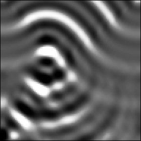
extrapolation in (![]() ,x,z)-space. At the top boundary data are
given as if recorded from a spherically diverging wave coming from
within the medium. The goal of this exercise is to show that the
(
,x,z)-space. At the top boundary data are
given as if recorded from a spherically diverging wave coming from
within the medium. The goal of this exercise is to show that the
(![]() ,x,z)-space can be used for downward extrapolation of
recorded data. The following is a listing of the existing program written
in ratfor. It is directly included from the directory in which this document
is stored.
,x,z)-space can be used for downward extrapolation of
recorded data. The following is a listing of the existing program written
in ratfor. It is directly included from the directory in which this document
is stored.
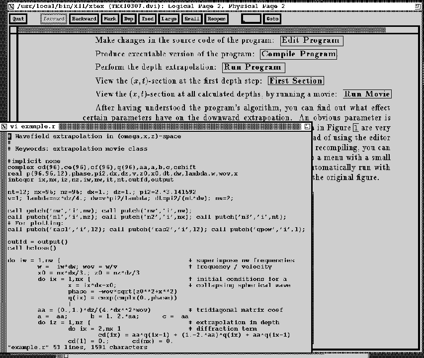
# Wavefield extrapolation in (omega,x,z)-space # # Keywords: extrapolation movie class#implicit none complex cd(96),ce(96),cf(96),q(96),aa,a,b,c,cshift real p(96,96,12),phase,pi2,dx,dz,v,z0,x0,dt,dw,lambda,w,wov,x integer ix,nx,iz,nz,iw,nw,it,nt,outfd,output
nt=12; nx=96; nz=96; dx=1.; dz=1.; pi2=2.*3.141592 v=1; lambda=nz*dz/4.; dw=v*pi2/lambda; dt=pi2/(nt*dw); nw=2;
call getch('nw','i',nw); call putch('nw','i',nw); call putch('n1','i',nz); call putch('n2','i',nx); call putch('n3','i',nt); # For plotting: call putch('ras1','i',12); call putch('ras2','i',12); call putch('gpow','i',1);
outfd = output() call hclose()
do iw = 1,nw { # superimpose nw frequencies w = iw*dw; wov = w/v # frequency / velocity x0 = nx*dx/3.; z0 = nz*dz/3 do ix = 1,nx { # initial conditions for a x = ix*dx-x0; # collapsing spherical wave phase = -wov*sqrt(z0**2+x**2) q(ix) = cexp(cmplx(0.,phase)) } aa = (0.,1.)*dz/(4.*dx**2*wov) # tridiagonal matrix coef a = -aa; b = 1.+2.*aa; c = -aa do iz = 1,nz { # extrapolation in depth do ix = 2,nx-1 # diffraction term cd(ix) = aa*q(ix+1) + (1.-2.*aa)*q(ix) + aa*q(ix-1) cd(1) = 0.; cd(nx) = 0. call ctris(nx,-a,a,b,c,-c,cd,q,ce,cf) # Solves complex tridiagonal equations cshift = cexp(cmplx(0.,wov*dz)) do ix = 1,nx # shifting term q(ix) = q(ix) * cshift do it=1,nt { # evolution in time cshift = cexp(cmplx(0.,-w*it*dt)) do ix = 1,nx p(iz,ix,it) = p(iz,ix,it)+q(ix)*cshift } } } do it=1,nt do ix=1,nx call rite(outfd, p(1,ix,it), nz*4) call exit(0) stop; end
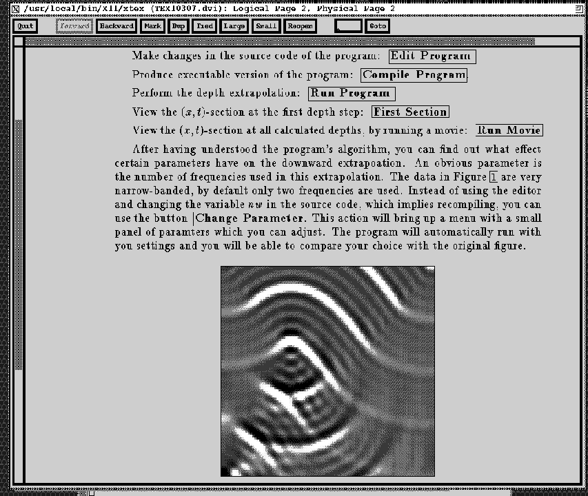
You are encouraged to make your own versions of this program by editing the file. Here are a few actions provided for you. To carry out the command, press the middle mouse button in the appropriate box:
Make changes in the source code of the program: Edit Program .sepsh>make Edit Program 
cake edit_example
Produce executable version of the program: Compile Program.sepsh>make Compile Program
cake compile_example
Perform the depth extrapolation: Run Program .sepsh>make Run Program
cake run_example
View the (x,t)-section at the first depth step: First Section.sepsh>make First Section
cake first_example
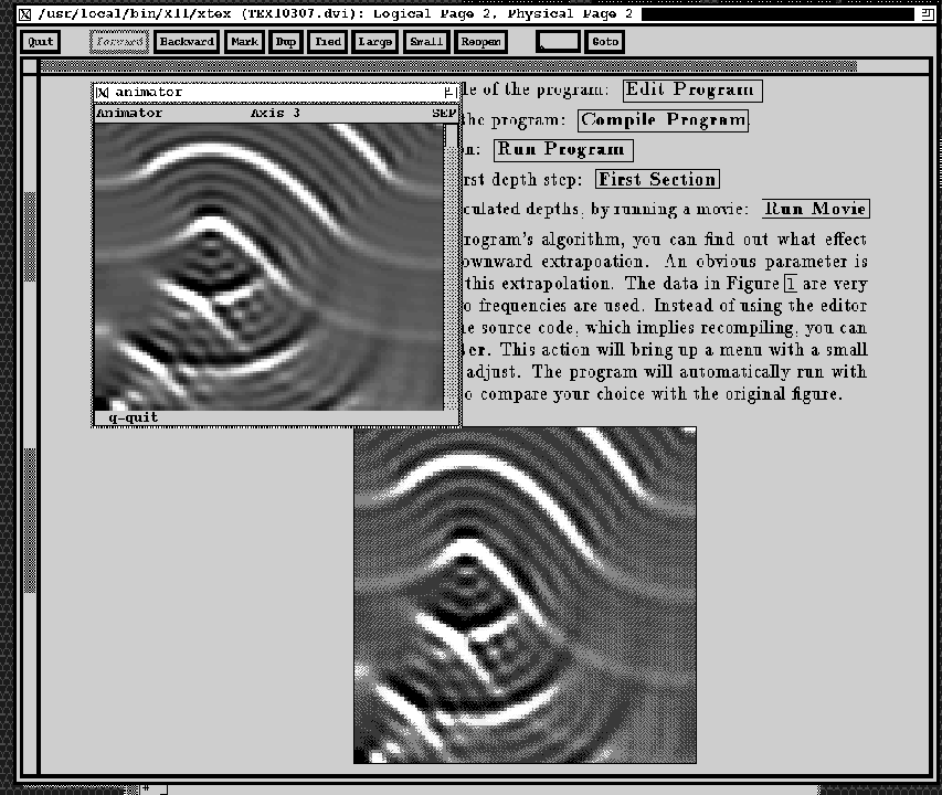
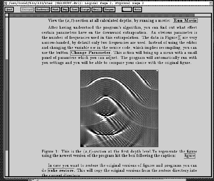
View the (x,t)-section at all calculated depths, by running a movie:
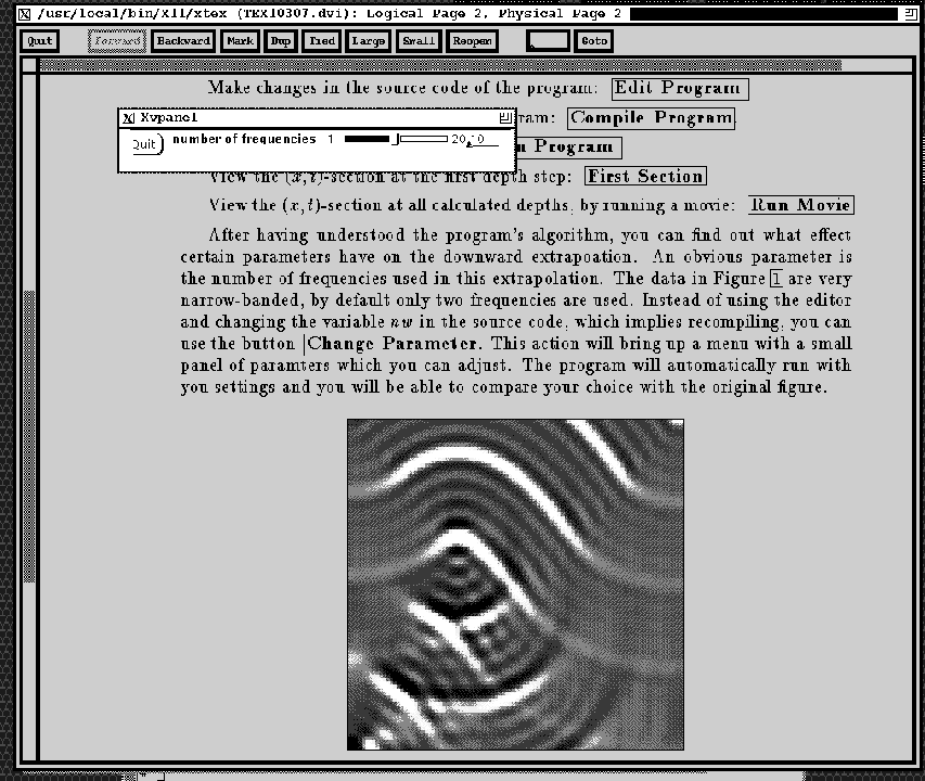
After having understood the program's algorithm, you can find out what effect certain parameters have on the downward extrapolation. An obvious parameter is the number of frequencies used in this extrapolation. The data in Figure 1 are very narrow-banded, by default only two frequencies are used. Instead of using the editor and changing the variable nw in the source code, which implies recompiling, you can use the button . This action will bring up a menu with a small panel of parameters which you can adjust. The program will automatically run with you settings and you will be able to compare your choice with the original figure.
 |

In case you want to restore the original versions of figures and programs you can do . This will copy the original versions from the restore directory into the current directory.
 |
 |
 |
 |
 |