


Next: EXAMPLES ON REAL DATA
Up: EXPRESSIONS OF THE PARABOLIC
Previous: Restrictions
Starting from a CMP-gather, we apply a NMO correction with the velocity
curve of the primaries, obtaining a data set d(t,h). Then, we apply
a Fourier transform in the time direction to transform the data set
to  . For each value of
  , we obtain the
field
, we obtain the
field  by solving the system:

This system is solved using Levinson algorithm, since the matrix LTWL
is Toeplitz. This property is independent of the weighting matrix W; it just
needs to be diagonal. It is also true for any spatial sampling.
We get the field U(t0,p) by applying the inverse Fourier in the time
direction. After having filtered the field U (for multiple removal, for
instance), we come back to the time-offset domain
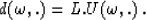
with the modeling operator L. To do so, we transform the field U to the
frequency domain, and for each frequency , we multiply it by the matrix
L (depending on ):
Finally, applying an inverse Fourier transform and an inverse NMO correction
brings us back to the original time-offset domain.
Next: EXAMPLES ON REAL DATA
Up: EXPRESSIONS OF THE PARABOLIC
Previous: Restrictions
Stanford Exploration Project
1/13/1998