Estimation of Q from surface-seismic reflection data in data space and image space

Forward modeling with Q

There are different models to describe Q: the Maxwell model, the Kelvin-Voigt model, the Zener model, the Burgers model, etc. Q behaves differently in the frequency domain in these different models. However, I use a nearly constant-Q model in this paper. The reason is that in oil prospecting and seismology, constant-Q models are convenient to parametrize attenuation in rocks, since the frequency dependence is usually not known. Moreover, there is physical evidence that attenuation is almost linear within the range of seismic frequencies, and thus the effect of Q is independent of these frequencies. Futterman (1962) has developed the theory for nearly constant Q, and I can use it in the forward modeling with Q.

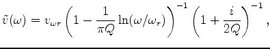
In Futterman's theory, the visco-acoustic equation has the same form as the acoustic equation, but the velocity is a complex number,

$$\tilde v(\omega ) = v_{\omega r} \left( {1 - \frac{1} {{\pi Q}}\l... ...omega /\omega _r )} \right)^{ - 1} \left( {1 + \frac{i} {{2Q}}} \right)^{ - 1},$$ (9)

where $\omega_r$ is the reference angular frequency, and $v_{\omega r}$ is the velocity at the reference angular frequency. Forward modeling can be executed with equation 9 using conventional one-way downward continuation, and more detailed algorithm is described in equations 11-16 in the following migration section.

I present a simple 2D synthetic example for the forward modeling. The model size is 4000 m (length) x 2500 m (depth). A horizontal reflector is at 1500 m depth. The source is located at x=0 on the surface, and 401 receivers are uniformly distributed along the surface. The medium is assumed to be homogeneous with constant velocity (2000 m/s) and constant Q (50 for the model with attenuation and 99999 for the model without attenuation). Injecting a Ricker wavelet produces the forward-modeled data in Figures 1(a) and 1(b). Their central frequencies are shown in Figures 1(c) and 1(d).

The wavelet in Figure 1(a) is stretched relative to the one in Figure 1(b), because the high frequency is attenuated more than the low frequency, which broadens the wavelet. Their central frequencies are also significantly different. Central frequency with attenuation in Figure 1(c) is a hyperbola along the offset, matching the theoretical calculation well. In contract, the central frequency is a flat line in Figure 1(d), indicating that no attenuation is accumulated along the ray path. Hence, Figures 1(c) and 1(d) provide further evidence that QVO carries information about attenuation and can be used to estimate Q.

Estimation of Q from surface-seismic reflection data in data space and image space