Estimation of Q from surface-seismic reflection data in data space and image space

Q migration

As with forward modeling, I use constant-Q assumption in Q migration. For convenience, I rewrite equation 9 in the form of slowness:

$$\tilde s(\omega ) = s_{\omega r} \left( {1 - \frac{1} {{\pi Q}}\ln (\omega /\omega _r )} \right)\left( {1 + \frac{i} {{2Q}}} \right),$$ (11)

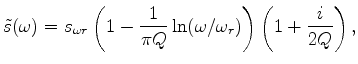
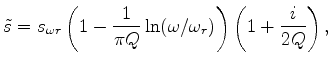
where $S_{\omega r}$ is the slowness at the reference frequency $\omega_r$ .

Having the new velocity/slowness, I obtain the new single square root as

$$\begin{gathered}k_z = {\text{SSR}}(\omega ,{\mathbf{k}}) \hfi... ...eft\vert {\mathbf{k}} \right\vert^2 }. \hfill \\ \end{gathered}$$ (12)

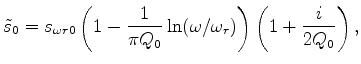
This new SSR can be approximated into a simplified form by using Taylor expansion around reference slowness $s_{0}$ and reference quality factor $Q_0$ :

$$\begin{gathered}k_z (s_{\omega r} ,Q) = k_{z0} (\tilde s_0 ) ... ...eft\vert {\mathbf{k}} \right\vert^2 }} \hfill\\ \end{gathered},$$ (13)

where

$$\tilde s = s_{\omega r} \left( {1 - \frac{1} {{\pi Q}}\ln (\omega /\omega _r )} \right)\left( {1 + \frac{i} {{2Q}}} \right),$$ (14)

$$\tilde s_0 = s_{\omega r0} \left( {1 - \frac{1} {{\pi Q_0 }}\ln (\omega /\omega _r )} \right)\left( {1 + \frac{i} {{2Q_0 }}} \right),$$ (15)

and $s_{\omega r}$ is the reference slowness at the reference frequency. The first two terms of equation 13 describe the split-step migration. The third term is the high-order correction, which allows for pseudo-screen migration.

The single square root for FFD migration is shown as follows:

$$\begin{gathered}k_z = k_z^{{\text{ref}}} + k_z^{{\text{split ... ...{\mathbf{k}} \right\vert} \right)^2 }}\hfill \\ \end{gathered},$$ (16)

where $a=0.5$ and $b=0.25$ for 45-degree migration.

In addition, I can rewrite Q migration in a matrix form to conveniently compare with the conventional migration. The conventional migration can be written in the following matrix form:

$$\begin{gathered}{\mathbf{d}} = {\mathbf{Fm}} \hfill \\ {\mathbf{m}} = {\mathbf{F}}^T {\mathbf{d}} \hfill \\ \end{gathered}$$ (17)

where $\bf {d}$ is the data, $\bf {m}$ is the model, $\bf {F}$ is the migration operator, and the superscript $T$ indicates the matrix transpose.

The downward continuation migration with Q can be written as

$$\begin{gathered}{\mathbf{d}} = {\mathbf{AFm}} \hfill \\ {\mat... ...hbf{F}}^T {\mathbf{A}}^T {\mathbf{d}} \hfill, \\ \end{gathered}$$ (18)

where $\bf {A}$ is the attenuation operator, which consists of real numbers less than $1$ .

Equation 18 indicates that the migrated model will be further attenuated, with the attenuation operator $\bf {A}$ being applied to the attenuated modeled data. Therefore, Q migration will compensate for the phase change, but will not compensate for the amplitude loss due to attenuation.

In this section, I apply Q migration to the modeled data in Figures 1(a) and 1(b). Figure 3(a) shows the conventional migration of the non-attenuated data in Figure 1(b), which images the reflector at 1500 m depth. Figures 3(b) and 3(c) show the conventional migration and Q migration of the attenuated data in Figure 1(a). The wavelets in Figure 3(c) are stretched in comparison to the ones in Figure 3(a). This result confirms that Q migration further attenuates the data, instead of compensating for its amplitude loss.

Estimation of Q from surface-seismic reflection data in data space and image space