next up previous [pdf]

Next: Conclusions Up: Model parametrization and sensitivity-kernel Previous: Velocity parametrization

Logarithmic velocity parametrization

A slightly different parametrization is to define $ {m_1=ln\left({v_p}^{-2}\right)}$ and $ {m_2=1+2\epsilon}$ 
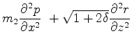
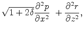
. Using this parametrization, equation 1 can be rewritten as follows:
$\displaystyle e^{m_1}\frac{\partial^2 p}{\partial t^2}$ $\displaystyle =$ $\displaystyle m_2\frac{\partial^2 p}{\partial x^2} \
+ \sqrt{1+2\delta}\frac{\partial^2 r}{\partial z^2}$  
$\displaystyle e^{m_1}\frac{\partial^2 r}{\partial t^2}$ $\displaystyle =$ $\displaystyle \sqrt{1+2\delta}\frac{\partial^2 p}{\partial x^2} \
+ \frac{\partial^2 r}{\partial z^2},$ (9)

Using a procedure similar to the one described in the previous section, we can obtain a matrix form expression:
$\displaystyle \begin{vmatrix}{ e^{m_{1,0}}\frac{\partial^2 }{\partial t^2} - m_...
...left\vert\begin{array}{c} {\Delta{m_1}} \\ {\Delta{m_2}}\end{array}\right\vert,$     (10)

This is the linear relationship between model perturbation and data perturbation, and can be used to calculate the sensitivity kernel. Figure 7 shows relative sensitivity kernel of the two model parameters. Both figures are clipped to the same value. With this parametrization, updates of both variables are of the same order of strength. I show in another paper [citation] that such parametrization results in very good inversion results.

relimpp
relimpp
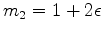
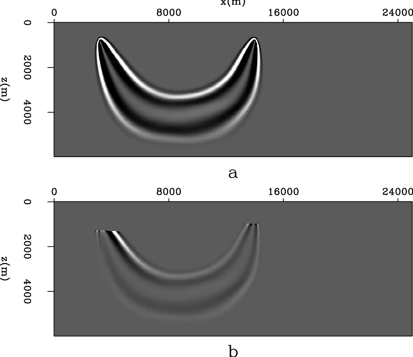
Figure 7.
Relative sensitivity kernel of parameter: a) $ {a^{-1}\ln\left({v_p}^{-2}\right)}$ ; b) $ {\left (1+2\epsilon \right )}$ . Both figures are clipped at the same value.
[pdf] [png]


next up previous [pdf]

Next: Conclusions Up: Model parametrization and sensitivity-kernel Previous: Velocity parametrization

2012-05-10