Early-arrival waveform inversion for near-surface velocity and anisotropic parameters: modeling and sensitivity kernel analysis

Model parametrization and sensitivity-kernel calculation

For inversion, there are several ways to parametrize the model space, which contains vertical p-wave velocity and the anisotropic parameters ${\epsilon }$ and ${\delta }$ . However, due to insensitivity of the data to the ${\delta }$ parameter, currently I consider a model space consisting of only vertical p-wave velocity and ${\epsilon }$ ; i.e. ${\delta }$ is fixed during inversion. Using gradient-based inversion methods, different parametrization leads to different model updates. In joint inversion, it is unfavorable to have updates that result in little or almost no change in one of the model components. Quantitatively, for a model space that contains two components ${m_1}$ and ${m_2}$ , update directions ${g_{m1}}$ and ${g_{m2}}$ should be chosen such that ${g_{m1}/m_1\approx{g_{m2}/m_{2}}}$ . This can be achieved by using proper parametrization.

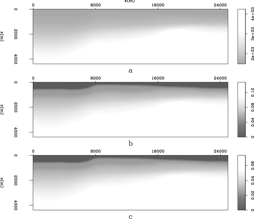
I compare three different parametrizations and their corresponding model updates (sensitivity kernels). For sensitivity-kernel calculation, I first calculate the full data residual by subtracting ${d_{cal}}$ , which is modeled from the smoothed version of the true model (Figure 4) from ${d_{obs}}$ , which is modeled from the true model. I consider only a single trace refraction of the total data residual for this study.

modelsbw
Figure 4. Smooth model for generating ${d_{cal}}$ : a) velocity model; b) ${\epsilon }$ model; c) ${\delta }$ model.

Early-arrival waveform inversion for near-surface velocity and anisotropic parameters: modeling and sensitivity kernel analysis