|
 |
 |
 | VTI migration velocity analysis using RTM |  |
![[pdf]](icons/pdf.png) |
Next: Numerical test
Up: Migration Velocity Analysis Gradients
Previous: Physical interpretation and implementation
Velocity model building is a highly underdetermined and nonlinear problem.
Therefore, prior knowledge of the subsurface is needed to define a
plausible subsurface model. In the formulation of Tarantola (1984),
prior information is included as the covariance and the mean of the model.
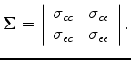
In this study, we assume the initial model we use is the mean, and the covariance
of the model has two independent components: spatial covariance and collocated
cross-parameter covariance (Li et al., 2011). In practice, instead of regularizing
the inversion using Tarantola (1984), we use a preconditioning scheme (Claerbout, 2009):
smoothing filtering to approximate square-root of the spatial covariance,
and a standard-deviation matrix to approximate the square-root of the cross-parameter covariance.
Mathematically, the preconditioned model perturbation  of the subsurface is defined as follows:
 |
(37) |
where
![$ {\bf m} = [c ~ \epsilon]^T$](img137.png) .
The smoothing operator
.
The smoothing operator  is a diagonal matrix:
 |
(38) |
with different smoothing operators for velocity and  , according to
the geological information in the study area.
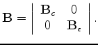
The standard deviation matrix
, according to
the geological information in the study area.
The standard deviation matrix  :
:
 |
(39) |
can be obtained by rock-physics modeling and/or lab measurements (Bachrach et al., 2011; Li et al., 2011).
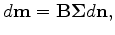
We call  the preconditioning variable, and it
relates to the original model
the preconditioning variable, and it
relates to the original model  as follows:
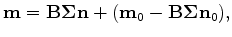 |
(40) |
where  and
and  are the initial models in preconditioned space and physical
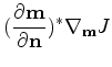
space, respectively. Now, the gradient of the objective function 15 with respect to
this preconditioning variable
is
are the initial models in preconditioned space and physical
space, respectively. Now, the gradient of the objective function 15 with respect to
this preconditioning variable
is
where
![$ \nabla_{\bf m} J = [\nabla_{c} J ~ \nabla_{\epsilon} J]^T$](img150.png) .
.
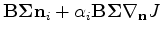
In a steepest-decent inversion framework, the initial preconditioning model
is obtained
by minimizing the following objective function:
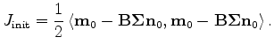 |
(42) |
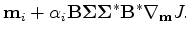
For the  iteration
 |
(43) |
Equation 44 suggests an interesting consideration in the context of nonlinear inversion: left-multiplying
the gradient with a (semi)positive-definite matrix is equivalent to preconditioning with the square-root of the matrix;
thus, the resulting direction is still a descent direction (Claerbout, 2009).
|
|
|
|
| VTI migration velocity analysis using RTM | |
|
Next: Numerical test
Up: Migration Velocity Analysis Gradients
Previous: Physical interpretation and implementation
2012-05-10