|
|
|
|
Fast velocity model evaluation with synthesized wavefields |
The procedure for Born modeling and migration to quickly test velocity models is detailed in Halpert and Tang (2011). To summarize, the major steps of the process are:
 |
(1) |
 are the arbitrarily defined locations where the wavefield will be recorded;
 is the vector of subsurface half-offsets;
  is angular frequency;
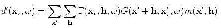
  is the initial image from which data is injected at isolated regions defined by
 ; and
; and  is the Green's function propagating the wavefield to the receiver locations (here,
  denotes the adjoint). Because the wavefield can be recorded at arbitrary locations, this method provides a simple means of re-datuming, which can lead to significant computational savings.
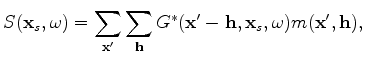
 and record it at arbitrary receiver locations
 :
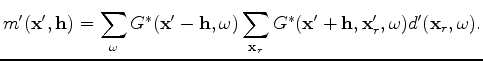
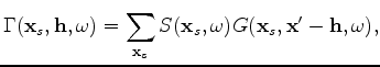
is the reflectivity model (in our case, the isolated regions from the initial image), and the
:
is the reflectivity model (in our case, the isolated regions from the initial image), and the  term is defined as
 |
(3) |
 is the source function described in step 1. Because the velocity model used to compute the Green's functions is the same one used to generate the initial image, the resulting Born-modeled wavefield
 will be kinematically invariant regardless of the initial model (Tang, 2011). This is important because the initial model will inevitably contain errors, and the goal of the procedure described here is to improve upon it.
With the procedure outlined above, significant savings may be realized if only a single shot is migrated, a situation made possible by the fact that an areal source function is used along with an arbitrary acquisition geometry. However, in many cases an image obtained in this manner is contaminated by crosstalk artifacts. Various solutions to the crosstalk attenuation problem have been proposed, for example using multiple phase-encoded shots (Tang, 2008; Romero et al., 2000). Unfortunately, this approach would hinder the computational efficiency of the evaluation procedure - one of its primary considerations. Instead, the procedure described above is applied only to isolated locations from a single reflector in the initial image. As long as these locations are separated by at least twice the maximum subsurface offset value used to synthesize the new source and receiver wavefields, any crosstalk problems should be avoided. This method also allows an interpreter or model-builder to select reflectors he or she thinks would be most sensitive to changes in the velocity model - for example, the base of salt.
|
|
|
|
Fast velocity model evaluation with synthesized wavefields |